Clustering and Tracking

Clustering

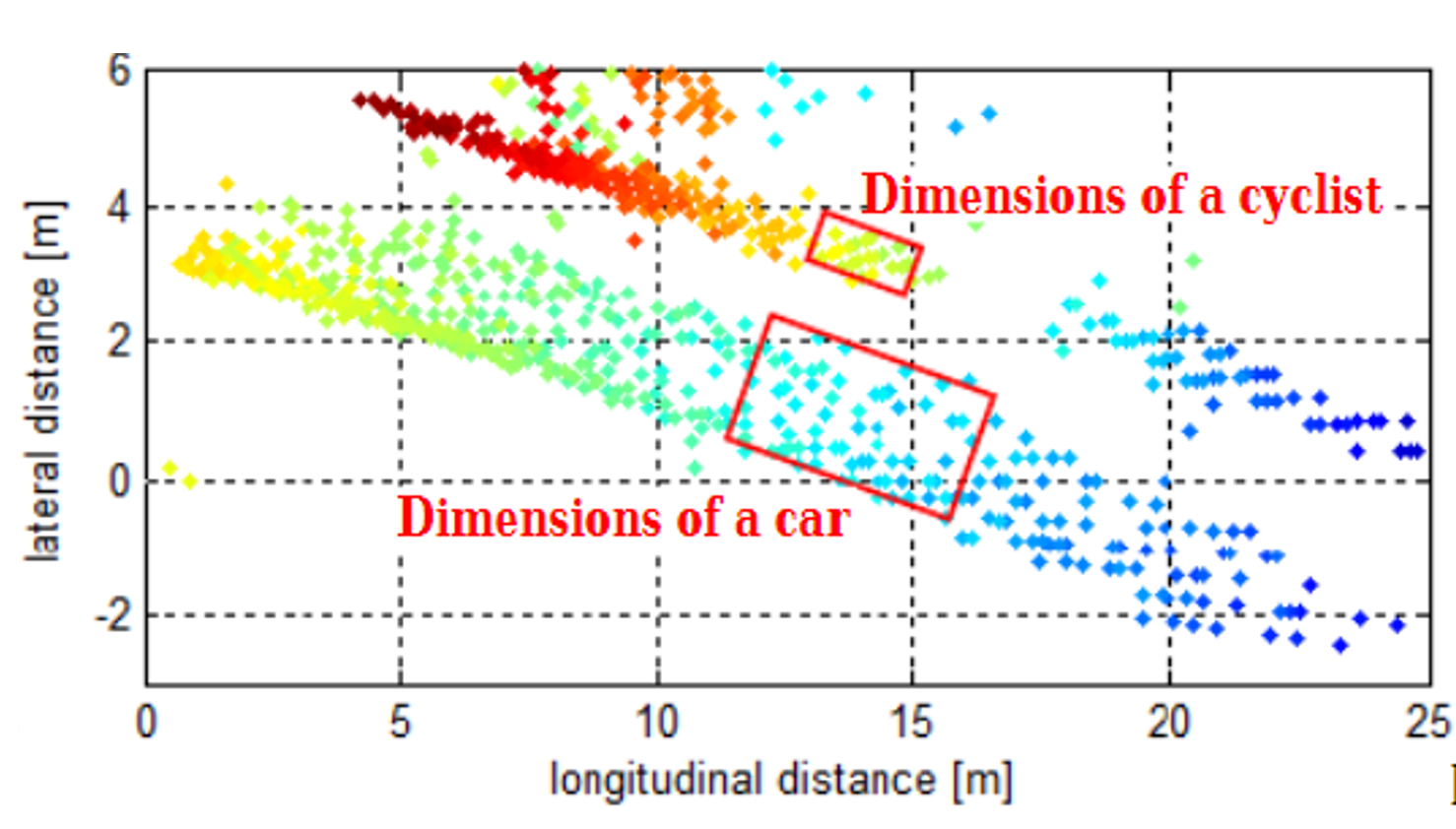
For enhanced perception in autonomous driving, there is a need to track multiple targets separately. The object tracking is computationally expensive and tracking multiple targets simultaneously requires lots of processing power and memory.

Due to the advancements in radar technology and increasing sensing resolutions, a radar can generate detections from plenitude of scattering points on the target. If a tracker is assigned to every detection from the same target, then it can overburden the processing unit. Hence, it is important to cluster the detections from every target and assign a single track for each.

This is where the clustering algorithm becomes important for successful object tracking.

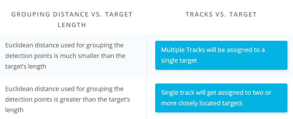
Here we will discuss the basic clustering algorithm based on the euclidean distance. The algorithm here groups the detection points based on their proximity measured by the euclidean distance between those points.

All the detection points that are within the size of the target are considered as one cluster, merged into a centroid position. Each cluster is now assigned a new range and velocity, which is the mean of measured range and velocity of all the detection points that form the cluster. This allows valid tracking for each target.

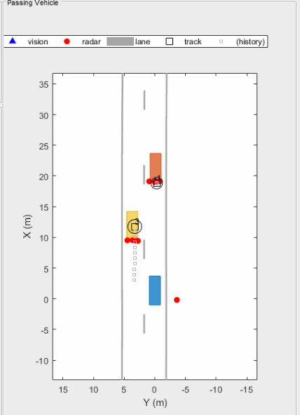
Above is an illustration of the clustering scenario. In the image the blue car is an ego vehicle (vehicle with sensor) and the detections are generated from the orange and yellow vehicles. Using clustering algorithm all the detections associated with the single target are merged into one point. This helps in the detection and assigning the tracks to a target.

Matlab Implementation of Clustering

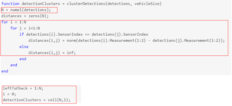
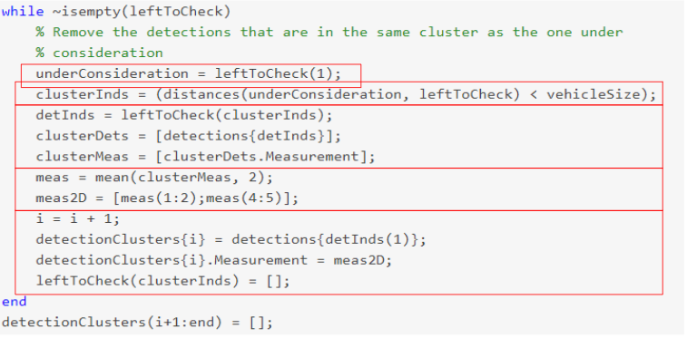
The clustering implementation above uses the following steps:

If the detections are from same sensor, then loop through every single detection point and measure the euclidean distance between all of them.

Keep running the loop until the detection list is empty

Implement the following within the while loop:

Pick the first detection in the check list and check for its clustering neighbors.

If the distance between the first pick and remaining detections is less than the vehicle size, then group those detections and their respective radar sensor measurements, including range and velocity.

For the group, take the mean of the range and velocity measurements.
Note: the radar measurement vector has 6 values - where range and velocity for x and y coordinates reside at indices 1,2, 4, and 5: [x, y, - , Vx, Vy, -]

Create a new Cluster ID. Then, assign all the group detections to the same ID.

Further, assign cluster, the mean range and velocity.

In the end, delete from the list the detections which have already been assigned to a cluster.

Keep repeating the process until the detection list is empty.

Kalman Tracking

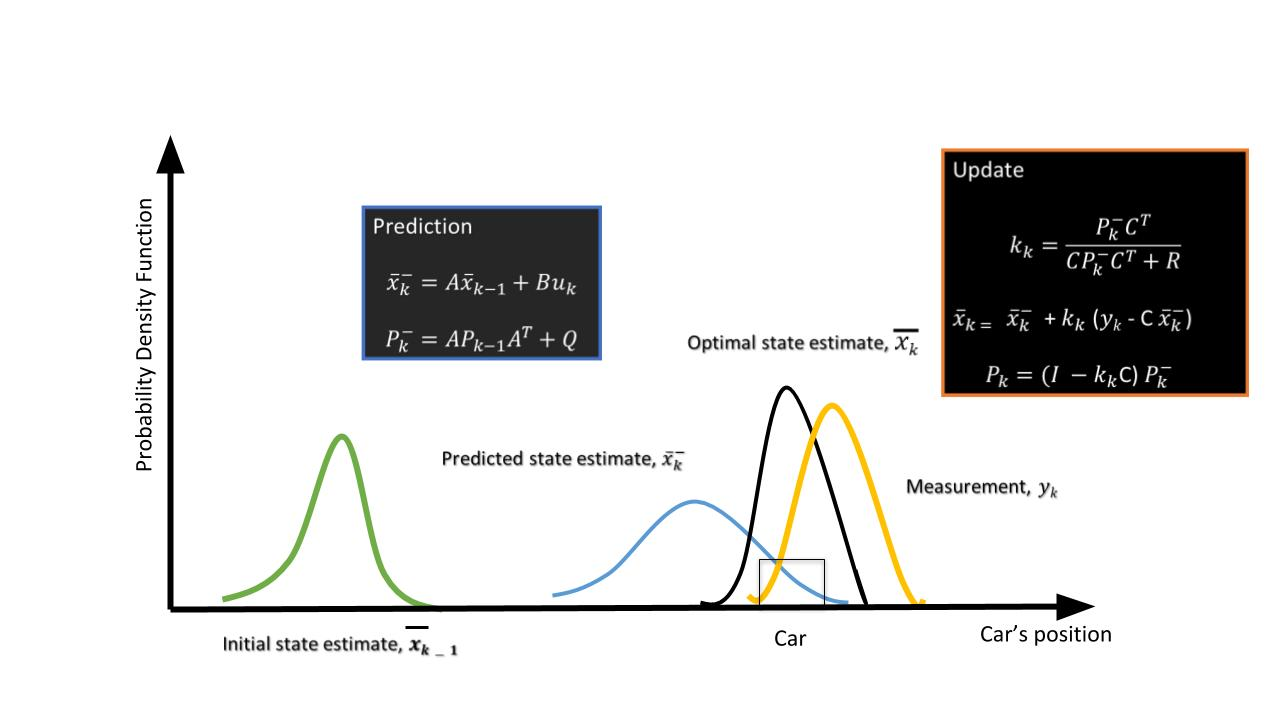
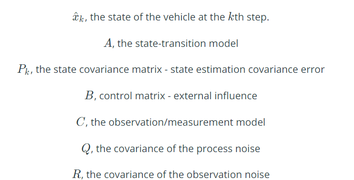
The purpose of the Kalman filter is to estimate the state of a tracked vehicle. Here, "state" could include the position, velocity, acceleration or other properties of the vehicle being tracked. The Kalman filter uses measurements that are observed over time that contain noise or random variations and other inaccuracies, and produces values that tend to be closer to the true values of the measurements and their associated calculated values. It is the central algorithm to the majority of all modern radar tracking systems.

Here, we will be keeping the Kalman Filter limited to a basic introduction. You will be covering Kalman filters in detail in the fourth course of this Nanodegree program.

The Kalman filter process has two steps: prediction and update.

Prediction Step Using the target vehicle's motion model, the next state of the target vehicle is predicted by using the current state. Since we know the current position and velocity of the target from the previous timestamp, we can predict the position of the target for next timestamp. For example, using a constant velocity model, the new position of the target vehicle can be computed as:

2. Update Step

Here, the Kalman filter uses noisy measurement data from sensors, and combines the data with the prediction from the previous step to produce a best-possible estimate of the state.

Kalman Tracking and MATLAB

The trackingKF class creates a discrete-time linear Kalman filter used for tracking positions and velocities of objects which can be encountered in an automated driving scenario, such as automobiles, pedestrians, bicycles, and stationary structures or obstacles.

You can learn more about different parameters for the filter here:

You can learn more about the theory behind Kalman filters here:

Implementation in MATLAB

The following guidelines can be used to implement a basic Kalman filter for the next project.

You will define the Kalman filter using the trackingKF function. The function signature is as follows:

filter = trackingKF('MotionModel', model, 'State', state, 'MeasurementModel', measurementModel, 'StateCovariance', stateCovrariance, 'MeasurementNoise', measurementNoise)

In this function signature, each property (e.g. 'MotionModel) is followed by the value for that property (e.g. model).

For the model variable, you can pass the string '2D Constant Velocity', which will provides the 2D constant velocity motion model.

For the 2D constant velocity model the state vector (x) can be defined as:

[x;vx;y;vy]
% Here, x and y are 2D position coordinates. The variablesvx and vy provide the velocity in 2D.

A RadarDetectionGenerator function is used to generate detection points based on the returns after reflection. Every Radar detection generates a detection measurement and measurement noise matrix: detection.Measurement and detection.MeasurementNoise. The detection measurement vector (z) has the format [x;y;vx;vy].

Measurement Models

Measurements are what you observe about your system. Measurements depend on the state vector but are not always the same as the state vector. The measurement model assumes that the actual measurement at any time is related to the current state by

z = H*x;

As a result, for the case above the measurement model is

H = [1 0 0 0; 0 0 1 0; 0 1 0 0; 0 0 0 1];

Using this measurement model, the state can derived from the measurements.

x = H'*z;
state = H'*detection.Measurement;

Further, using the generated measurement noise and measurement model define the state covariance matrix:

stateCovariance =H'*detection.MeasurementNoise*H;

Further Research

For further explanation of Kalman Filters with MATLAB, you can refer to this video series.

MATLAB Sensor Fusion Guided Walkthrough

A guided walk-through of performing Kalman Filtering in a simulated environment using MATLAB. Starter code file Sensor_Fusion_with_Radar.m can be found on GitHub.

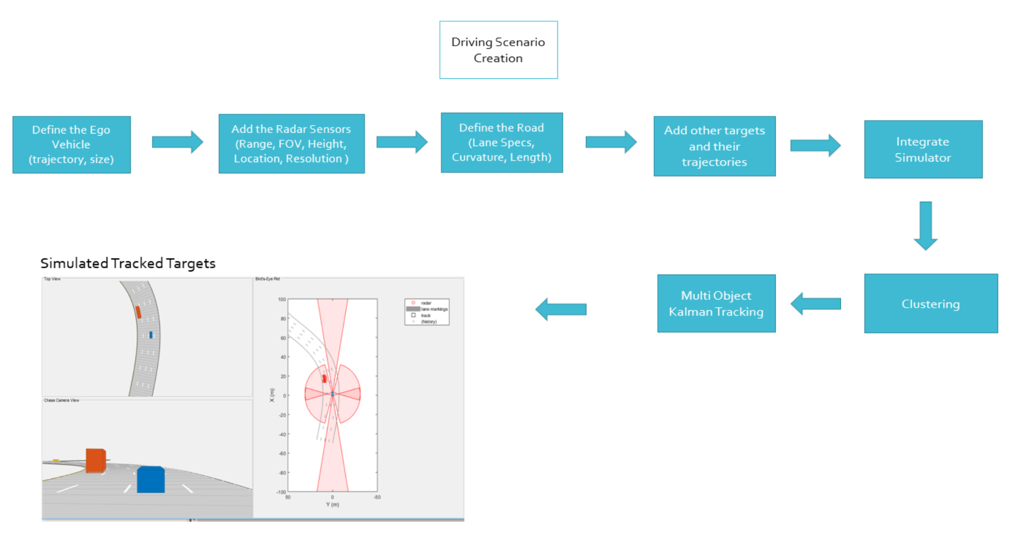
Sensor fusion and control algorithms for automated driving systems require rigorous testing. Vehicle-based testing is not only time consuming to set up, but also difficult to reproduce. Automated Driving System Toolbox provides functionality to define road networks, actors, vehicles, and traffic scenarios, as well as statistical models for simulating synthetic radar and camera sensor detection. This example shows how to generate a scenario, simulate sensor detections, and use sensor fusion to track simulated vehicles. The main benefit of using scenario generation and sensor simulation over sensor recording is the ability to create rare and potentially dangerous events and test the vehicle algorithms with them. This example covers the entire synthetic data workflow.

Scenario generation comprises generating a road network, defining vehicles that move on the roads, and moving the vehicles.In this example, you test the ability of the sensor fusion to track a vehicle that is passing on the left of the ego vehicle. The scenario simulates a highway setting, and additional vehicles are in front of and behind the ego vehicle. Find more on how to generate these scenarios here, Automated Driving Toolbox:

% Define an empty scenario

scenario = drivingScenario;
scenario.SampleTime = 0.01;

% Add a stretch of 500 meters of typical highway road with two lanes. % The road is defined using a set of points, where each point defines the center of the % road in 3-D space, and a road width.

roadCenters = [0 0; 50 0; 100 0; 250 20; 500 40];
roadWidth = 7.2; % Two lanes, each 3.6 meters
road(scenario, roadCenters, roadWidth);

% Create the ego vehicle and three cars around it: one that overtakes the ego vehicle % and passes it on the left, one that drives right in front of the ego vehicle and % one that drives right behind the ego vehicle. % All the cars follow the path defined by the road waypoints by using the path driving % policy. The passing car will start on the right lane, move to the left lane to pass, % and return to the right lane.% Create the ego vehicle that travels at 25 m/s along the road.
egoCar = vehicle(scenario, 'ClassID', 1);
path(egoCar, roadCenters(2:end,:) - [0 1.8], 25); % On right lane% Add a car in front of the ego vehicle.
leadCar = vehicle(scenario, 'ClassID', 1);
path(leadCar, [70 0; roadCenters(3:end,:)] - [0 1.8], 25); % On right lane% Add a car that travels at 35 m/s along the road and passes the ego vehicle.
passingCar = vehicle(scenario, 'ClassID', 1);
waypoints = [0 -1.8; 50 1.8; 100 1.8; 250 21.8; 400 32.2; 500 38.2];
path(passingCar, waypoints, 35);

% Add a car behind the ego vehicle
chaseCar = vehicle(scenario, 'ClassID', 1);
path(chaseCar, [25 0; roadCenters(2:end,:)] - [0 1.8], 25); % On right lane

Define Radar

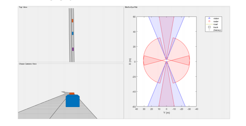
In this example, you simulate an ego vehicle that has 6 radar sensors covering the 360 degrees field of view. The sensors have some overlap and some coverage gap. The ego vehicle is equipped with a long-range radar sensor on both the front and the back of the vehicle. Each side of the vehicle has two short-range radar sensors, each covering 90 degrees. One sensor on each side covers from the middle of the vehicle to the back. The other sensor on each side covers from the middle of the vehicle forward. The figure in the next section shows the coverage.

sensors = cell(6,1);

% Front-facing long-range radar sensor at the center of the front bumper of the car.
sensors{1} = radarDetectionGenerator('SensorIndex', 1, 'Height', 0.2, 'MaxRange', 174, ...
 'SensorLocation', [egoCar.Wheelbase + egoCar.FrontOverhang, 0], 'FieldOfView', [20, 5]);

The rest of the radar sensors are defined in the project code.

Create a multiObjectTracker

Create a multiObjectTracker to track the vehicles that are close to the ego vehicle. The tracker uses the initSimDemoFilter supporting function to initialize a constant velocity linear Kalman filter that works with position and velocity. Tracking is done in 2-D. Although the sensors return measurements in 3-D, the motion itself is confined to the horizontal plane, so there is no need to track the height.

tracker = multiObjectTracker('FilterInitializationFcn', @initSimDemoFilter, ...
 'AssignmentThreshold', 30, 'ConfirmationParameters', [4 5]);

positionSelector = [1 0 0 0; 0 0 1 0]; % Position selector
velocitySelector = [0 1 0 0; 0 0 0 1]; % Velocity selector

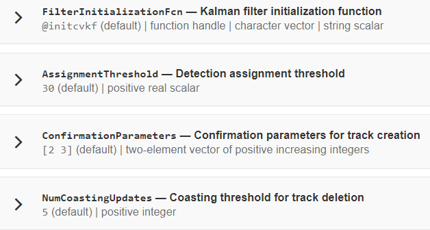
MultiObjectTracker Function has several parameters that can be tuned for different driving scenarios. It controls the track creation and deletion One can learn more about these

Simulate the Scenario

The following loop moves the vehicles, calls the sensor simulation, and performs the tracking. Note that the scenario generation and sensor simulation can have different time steps. Specifying different time steps for the scenario and the sensors enables you to decouple the scenario simulation from the sensor simulation. This is useful for modeling actor motion with high accuracy independently from the sensor’s measurement rate.

Another example is when the sensors have different update rates. Suppose one sensor provides updates every 20 milliseconds and another sensor provides updates every 50 milliseconds. You can specify the scenario with an update rate of 10 milliseconds and the sensors will provide their updates at the correct time. In this example, the scenario generation has a time step of 0.01 second, while the sensors detect every 0.1 second.

The sensors return a logical flag, isValidTime, that is true if the sensors generated detections. This flag is used to call the tracker only when there are detections. Another important note is that the sensors can simulate multiple detections per target, in particular when the targets are very close to the radar sensors. Because the tracker assumes a single detection per target from each sensor, you must cluster the detections before the tracker processes them. This is done by implementing clustering algorithm, the way we discussed above.

toSnap = true;
while advance(scenario) && ishghandle(BEP.Parent)    
    % Get the scenario time
    time = scenario.SimulationTime;

    % Get the position of the other vehicle in ego vehicle coordinates
    ta = targetPoses(egoCar);

    % Simulate the sensors
    detections = {};
    isValidTime = false(1,6);
    for i = 1:6
        [sensorDets,numValidDets,isValidTime(i)] = sensors{i}(ta, time);
        if numValidDets
            detections = [detections; sensorDets]; %#ok<AGROW>endend% Update the tracker if there are new detectionsif any(isValidTime)
        vehicleLength = sensors{1}.ActorProfiles.Length;
        detectionClusters = clusterDetections(detections, vehicleLength);
        confirmedTracks = updateTracks(tracker, detectionClusters, time);

        % Update bird's-eye plot
        updateBEP(BEP, egoCar, detections, confirmedTracks, positionSelector, velocitySelector);
    end
% Snap a figure for the document when the car passes the ego vehicle
if ta(1).Position(1) > 0 && toSnap
        toSnap = false;
        snapnow
    end
end

Define the Kalman Filter

Define the Kalman Filter here to be used with multiObjectTracker.

In MATLAB a trackingKF function can be used to initiate Kalman Filter for any type of Motion Models. This includes the 1D, 2D or 3D constant velocity or even constant acceleration. You can read more about this here.

initSimDemoFilter This function initializes a constant velocity filter based on a detection.

function filter = initSimDemoFilter(detection)
% Use a 2-D constant velocity model to initialize a trackingKF filter.
% The state vector is [x;vx;y;vy]
% The detection measurement vector is [x;y;vx;vy]
% As a result, the measurement model is H = [1 0 0 0; 0 0 1 0; 0 1 0 0; 0 0 0 1]

H = [1 0 0 0; 0 0 1 0; 0 1 0 0; 0 0 0 1];
filter = trackingKF('MotionModel', '2D Constant Velocity', ...
 'State', H' * detection.Measurement, ...
 'MeasurementModel', H, ...
 'StateCovariance', H’ * detection.MeasurementNoise * H, ...
 'MeasurementNoise', detection.MeasurementNoise);
end

Cluster Detections

This function merges multiple detections suspected to be of the same vehicle to a single detection. The function looks for detections that are closer than the size of a vehicle. Detections that fit this criterion are considered a cluster and are merged to a single detection at the centroid of the cluster. The measurement noises are modified to represent the possibility that each detection can be anywhere on the vehicle. Therefore, the noise should have the same size as the vehicle size. In addition, this function removes the third dimension of the measurement (the height) and reduces the measurement vector to [x;y;vx;vy].

We already went through its implementation in the clustering concept of this lesson.

📢

It is highly recommended to spend some time on this sensor fusion code. It’s a good place to start learning and implementing sensor fusion techniques.