Lidar and Radar Fusion with Kalman Filters in C++ (follow)
State Prediction
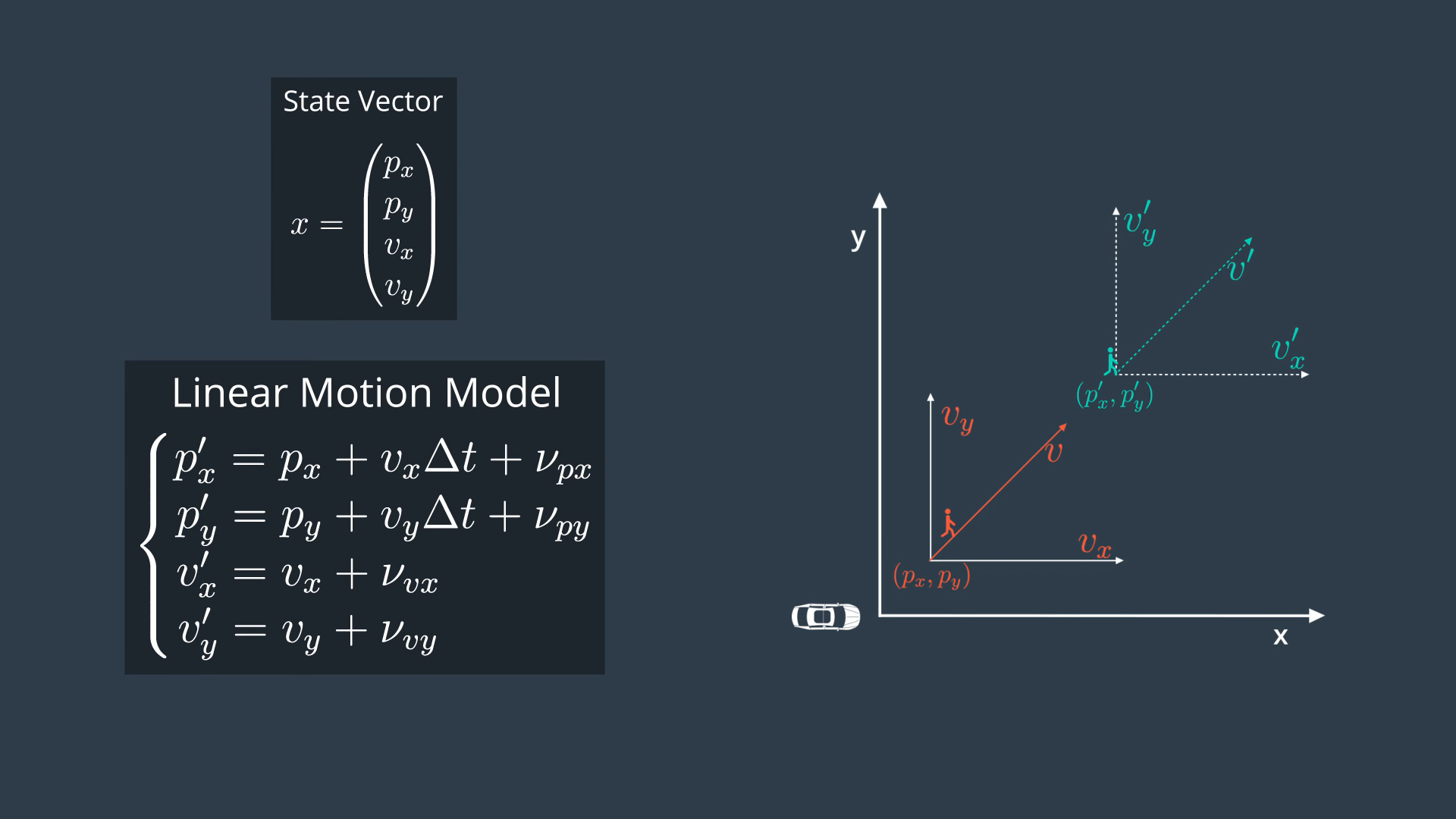
We are now in the prediction step. Since the pedestrian moves in both directions x and y, we need to define 2D position and 2D velocity, so we have 4D state vector. We also use the same linear motion model with constant velocity.
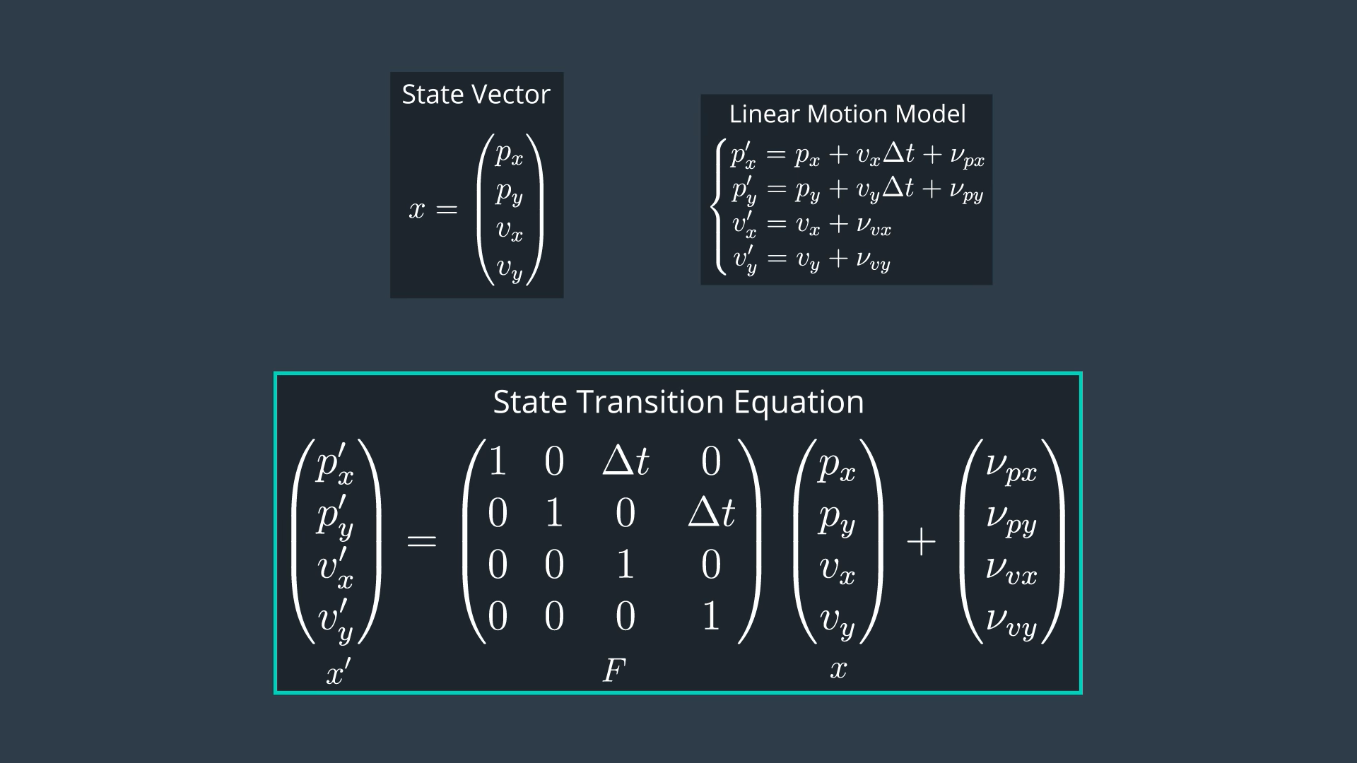
This gives us the following state transition matrix:
Also, the delta t is not constant any more. In reality, the time elapse between two consecutive observations might vary.
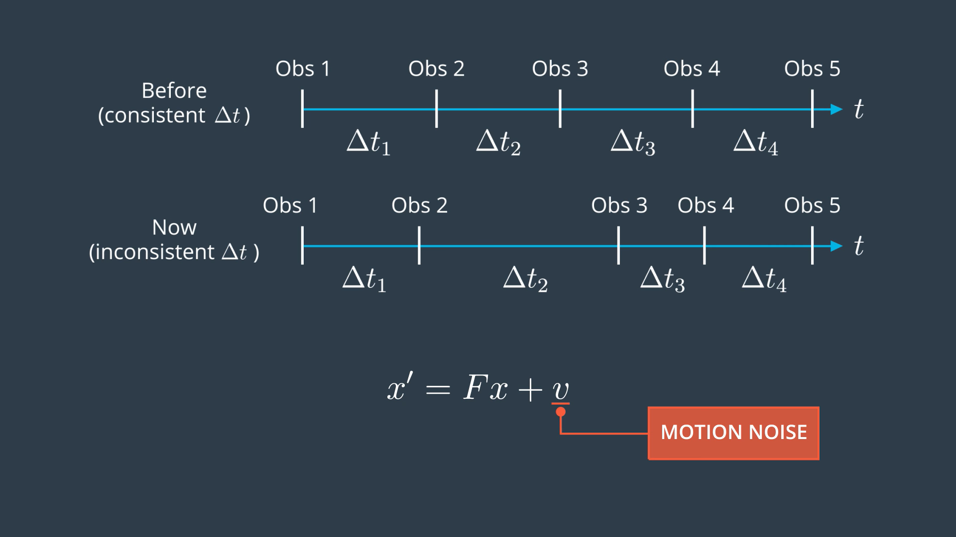
Motion noise and process noise refer to the same case: uncertainty in the object's position when predicting location. The model assumes velocity is constant between time intervals, but in reality we know that an object's velocity can change due to acceleration. The model includes this uncertainty via the process noise.
Measurement noise refers to uncertainty in sensor measurements, which will be discussed in more detail later.
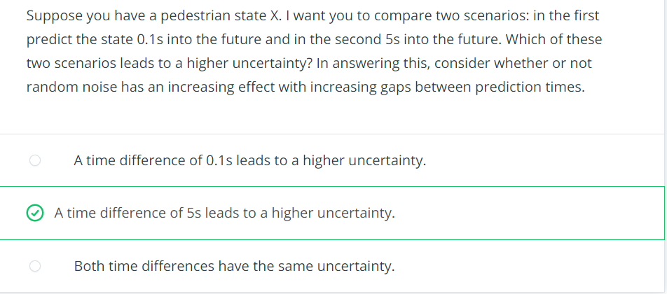
Here's another way of thinking about it: if you split the 5s time difference into several intermediate predictions with a difference of 0.1s, then compared to the first case, you will predict the same state many more times without receiving any feedback about the object's new position. Thus, the uncertainty increases.
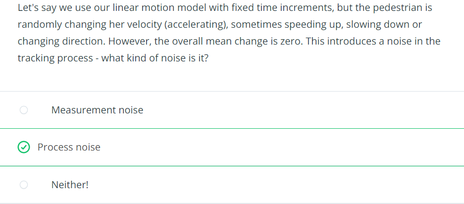
The prediction equation treats the pedestrian's velocity as constant. As such, a randomly accelerating pedestrian creates a process noise.
From the examples, we can clearly see that the process noise depends on both: the elapsed time and the uncertainty of acceleration. So, how can we model the process noise by considering both of these factors?
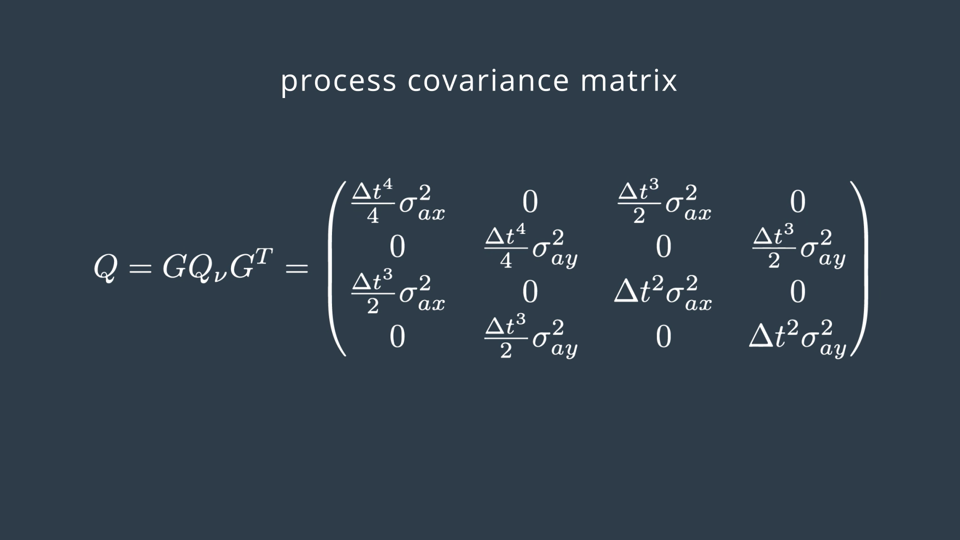
We need the process covariance matrix to model the stochastic of the state transition function.

First we explain how acceleration is expressed by kinematics equations. Second, we use that to derive process covariance matrix Q.
Say we have 2 consecutive observations of a pedestrian with initial and final velocities. From Kinematic formulas, we can derive the car position and speed as a function of previous state variables including change in velocity (acceleration).
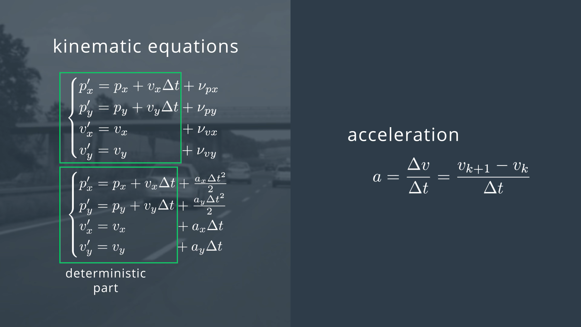
In the deterministic part of our motion model, we assume that the velocity is constant. However, in reality, pedestrian speed might change → But since acceleration is unknown, we can add it to noise component (expressed analytically in the last term of equation).
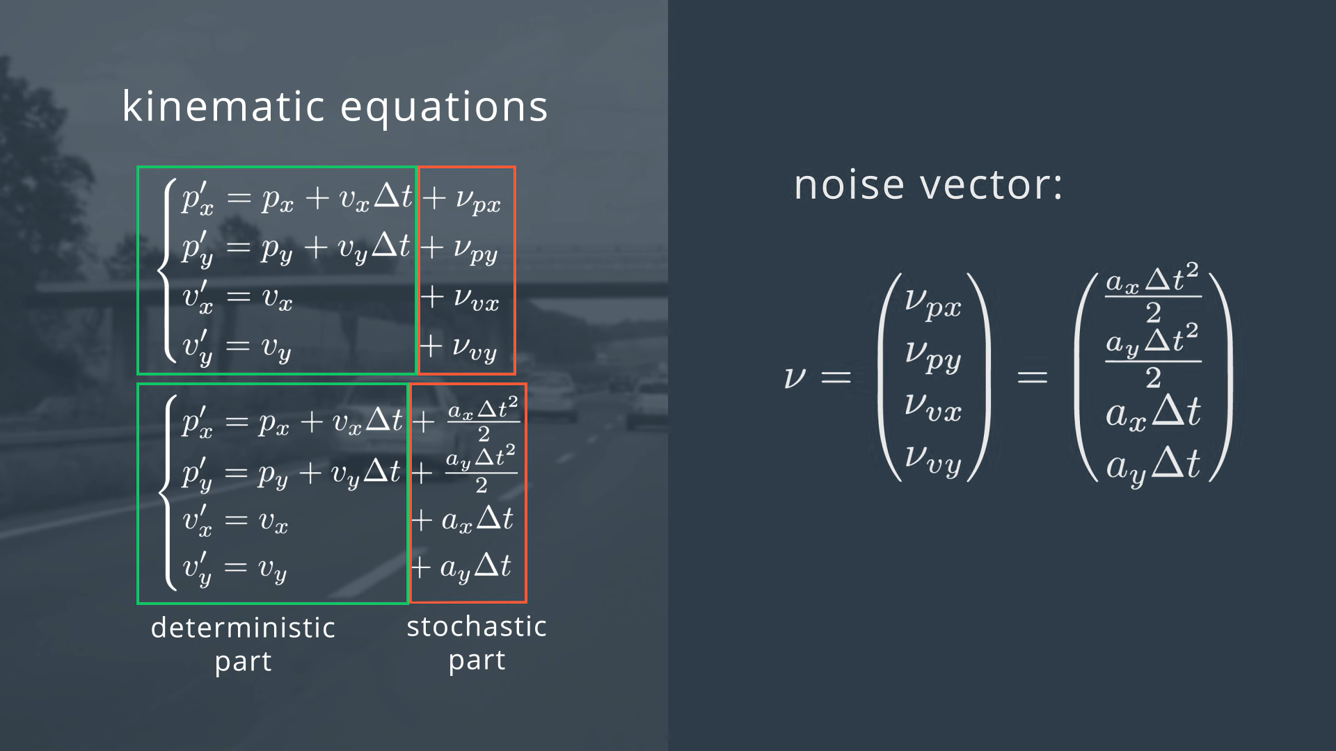
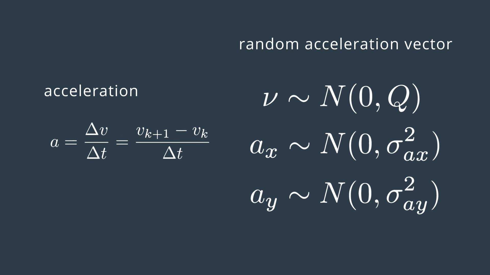
delta t is computed at each Kalman filter step, and the acceleration is a random vector with zero mean and standard deviation sigma.
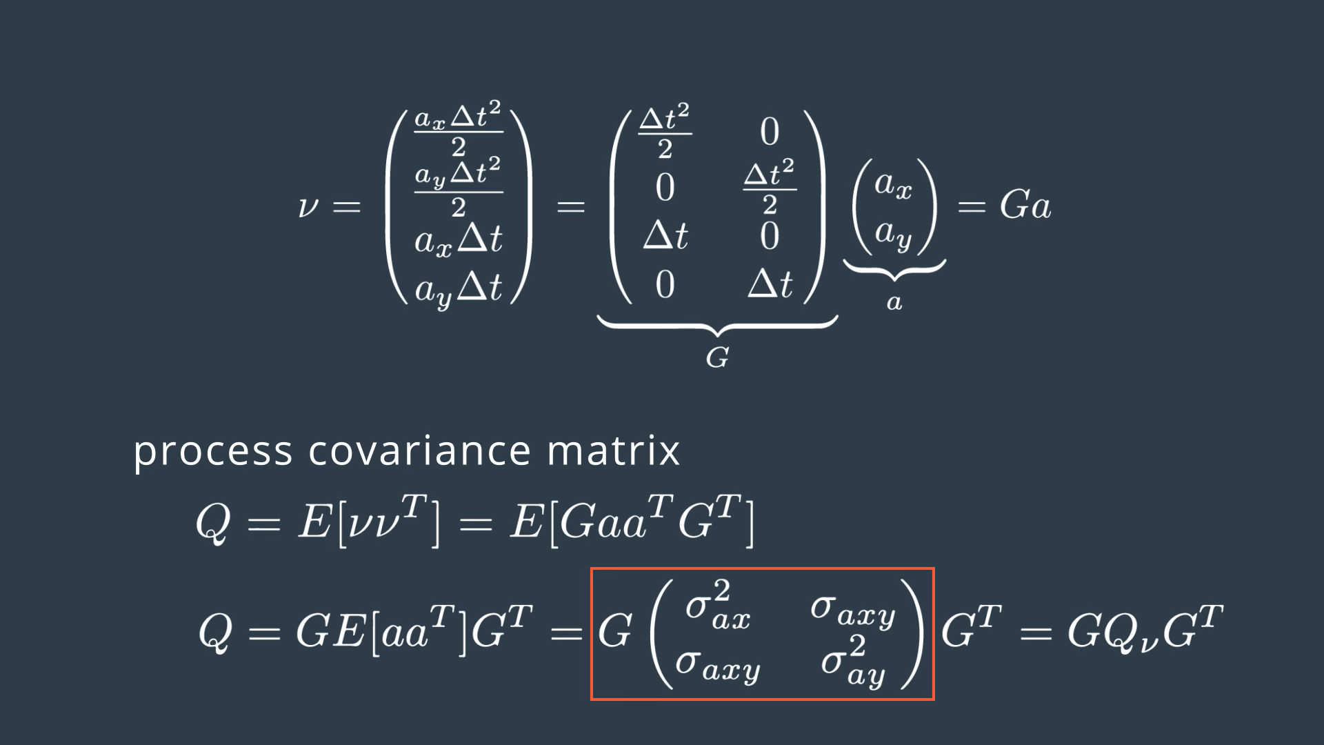
G: does not contain random variables
a: contains random acceleration components
v (mu): noise vector
Since G has no random variables, we can put it outside expectation calculation. This gives 3 statistical moments:
- Expectation of ax * ax → Variance of ax → sigma ax squared
- Expectation of ay * ay → Variance of ay → sigma ay squared
- Expectation of ax * ay → covariance of ax, ay → sigma axy
Note: ax and ay are assumed uncorrelated noise processes → Covariance = 0.
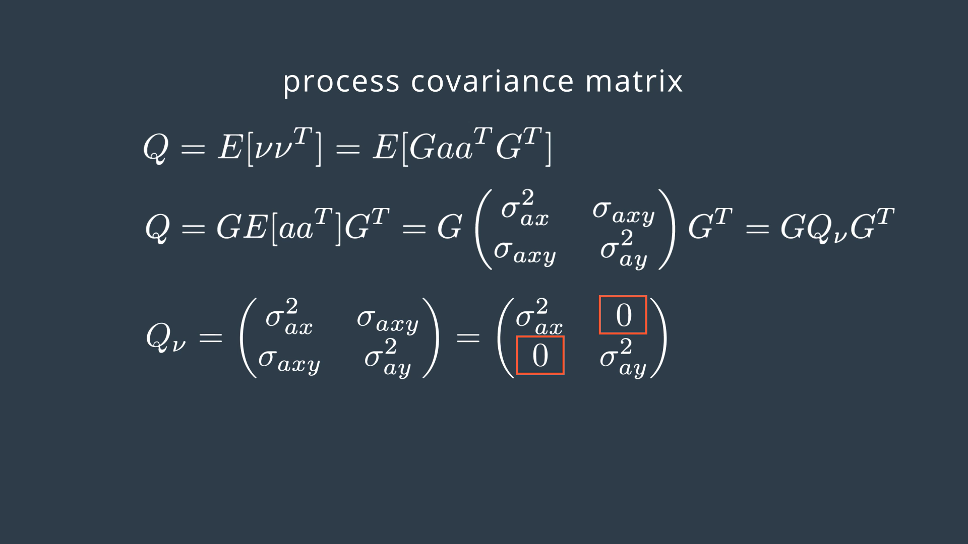
Combining everything together, we obtain:
Laser Measurements
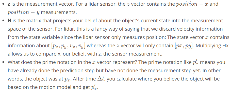
We have defined the motion model. Lets say a lidar measurement has come. Lets design our measurement model for a laser sensor in 2D. We need to define z, H, R.
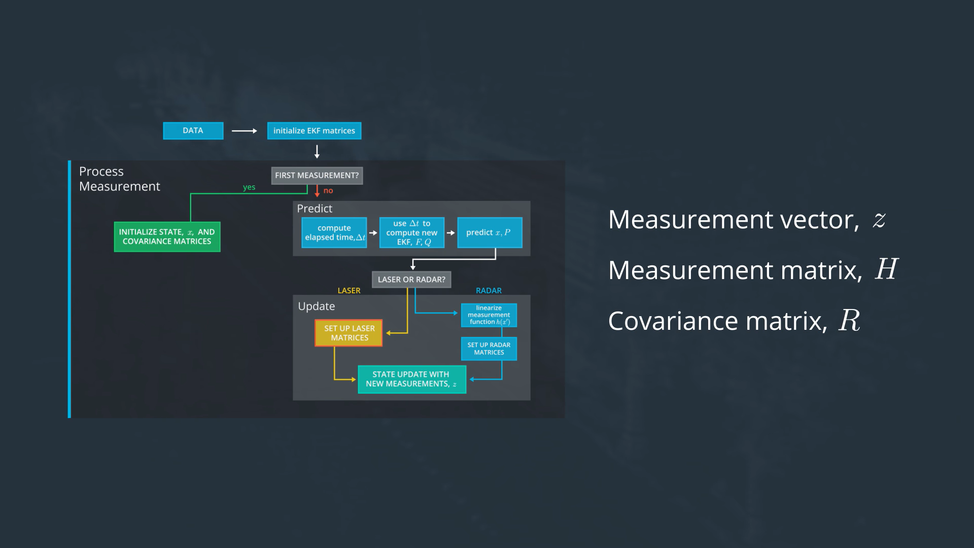
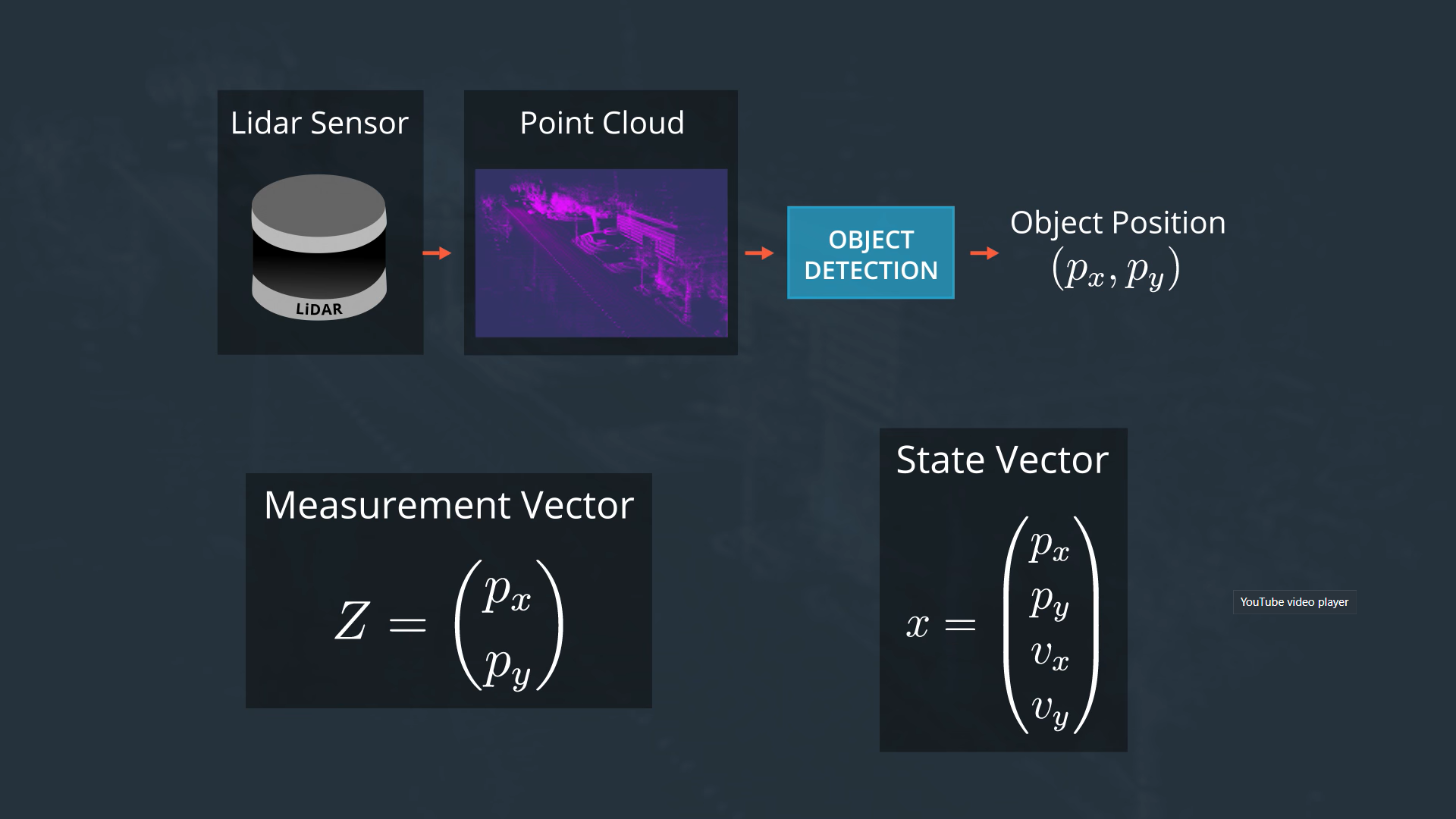
For simplicity we assume that we analyzed the point cloud to compute the 2D location of the pedestrian.
Measurement Noise Covariance Matrix R
Let's take a look at the covariance matrix, R, which represents the uncertainty in our sensor measurements. The dimensions of the R matrix is square and each side of its matrix is the same length as the number of measurements parameters. So, in our case here it is 2x2 matrix.
For laser sensors, we have a 2D measurement vector. Each location component px, py are affected by a random noise. So our noise vector ω has the same dimension as z. And it is a distribution with zero mean and a 2 x 2 covariance matrix which comes from the product of the vertical vector ω and its transpose.

where R is the measurement noise covariance matrix; in other words, the matrix R represents the uncertainty in the position measurements we receive from the laser sensor.

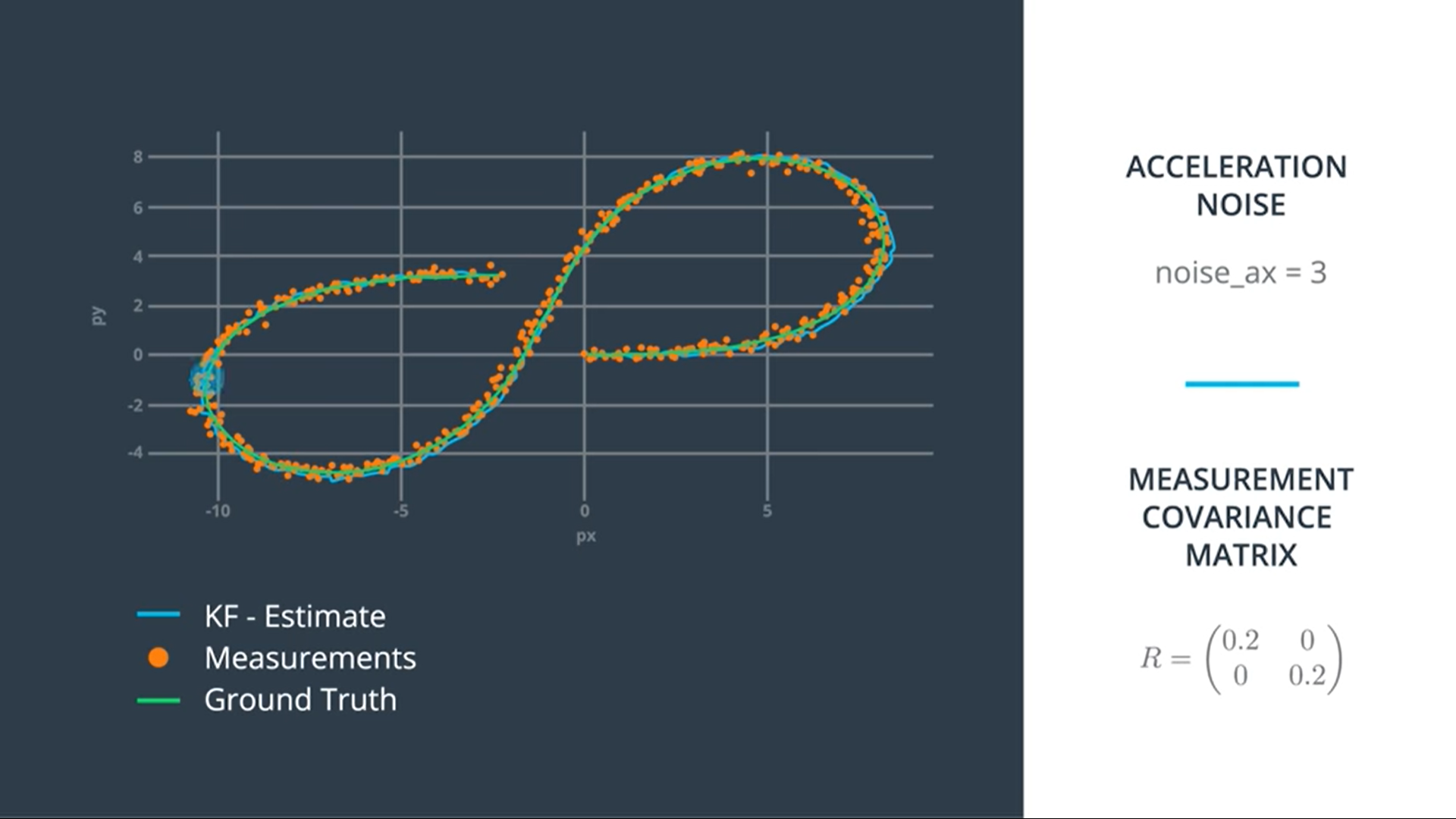
Here the sensor noise is low = 0.2, but if we increase measurement and process noises, the estimation changes:

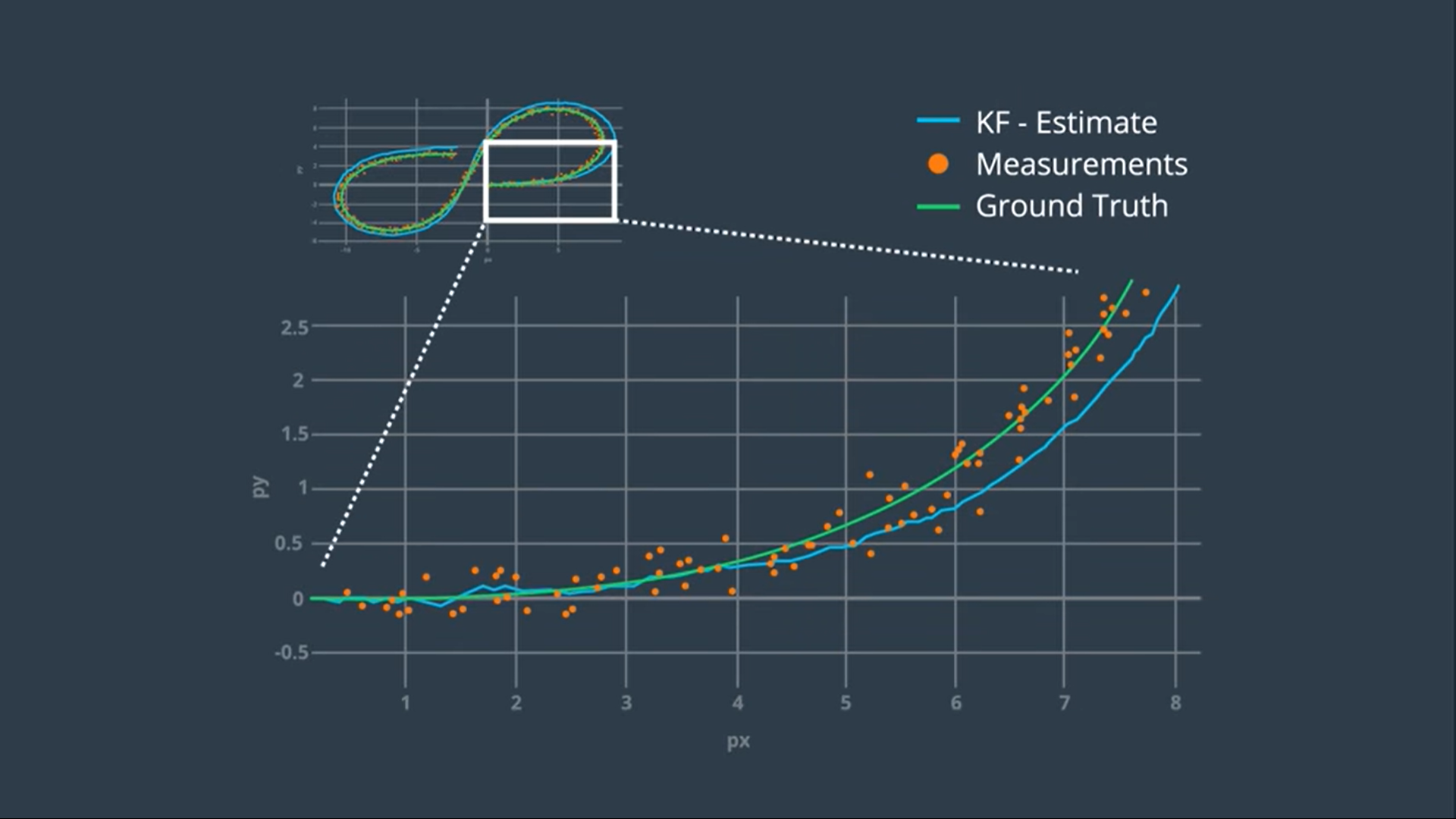
Our linear motion model is not perfect especially when the pedestrian moves on a circular path, as in our model, we always predict that the pedestrian position will be somewhat along a straight line. We can fix that by using a circular motion model instead of linear motion model.
More Info on Timestamps

Timestamps are often used for logging a sequence of events, so that we know exactly, for example, in our case when the measurements were generated.
We can use the timestamp values to compute the elapsed time between two consecutive observations as:
float delta_t = ( timestamp(k+1) - timestamp(k) ) / 1000000.0;Additionally we divide the result by 10^6 to transform it from microseconds to seconds.
float dt = (measurement_pack.timestamp_ - previous_timestamp_) / 1000000.0;Radar Measurements
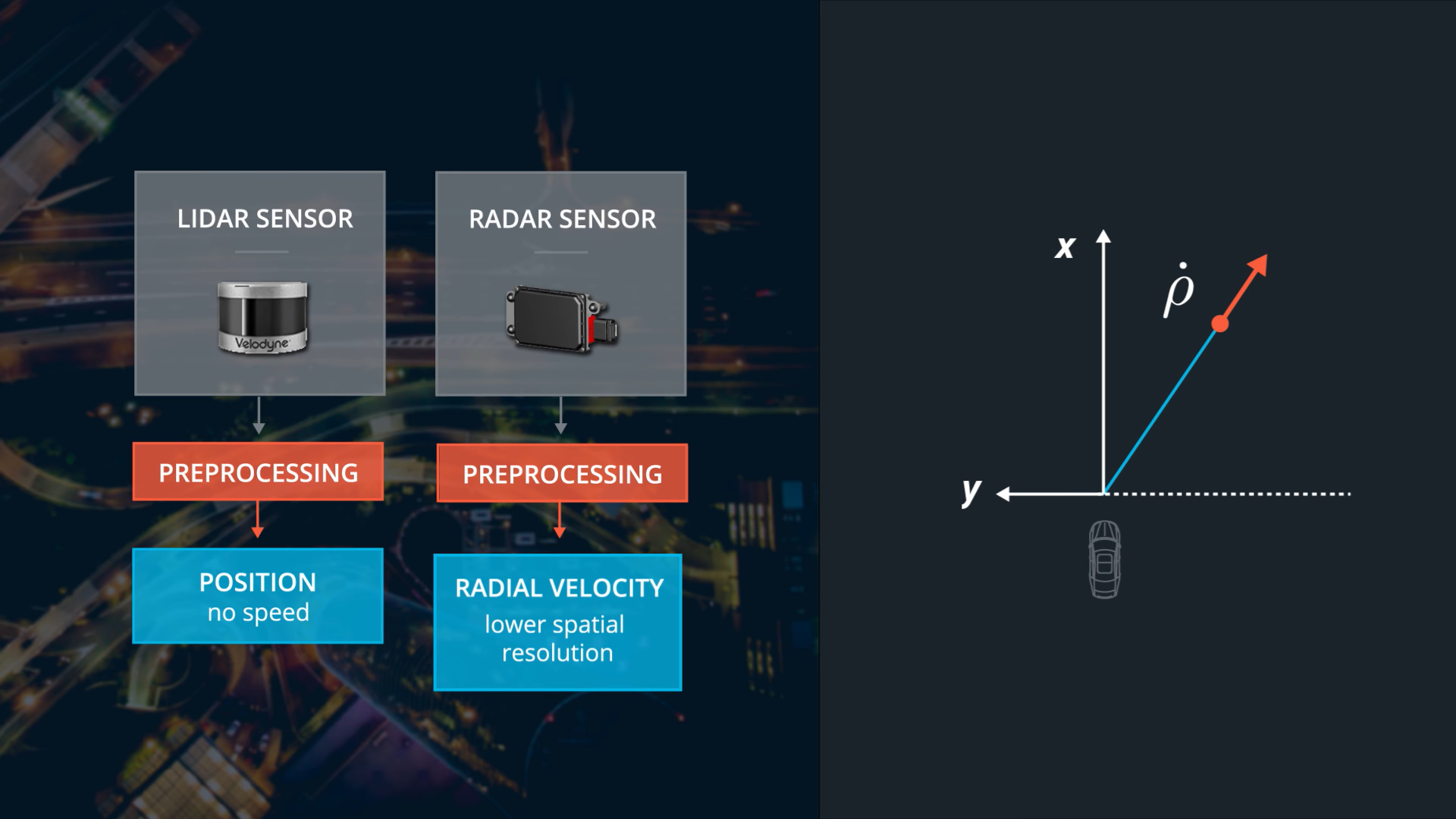
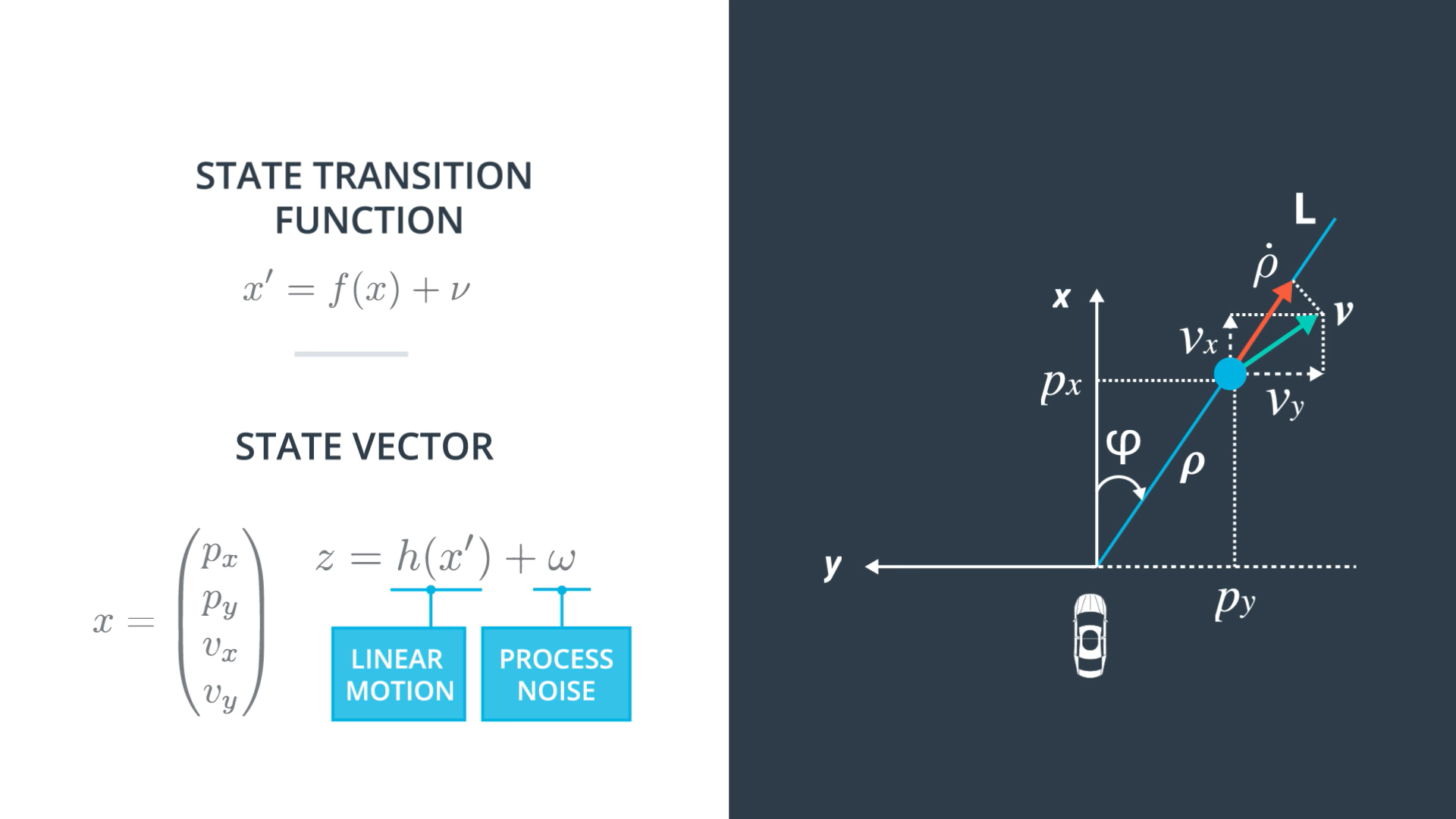
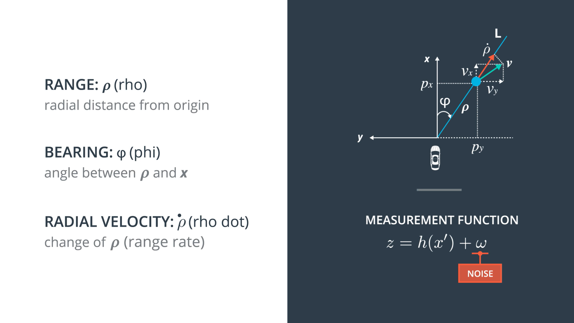
- X direction is the direction of motion.
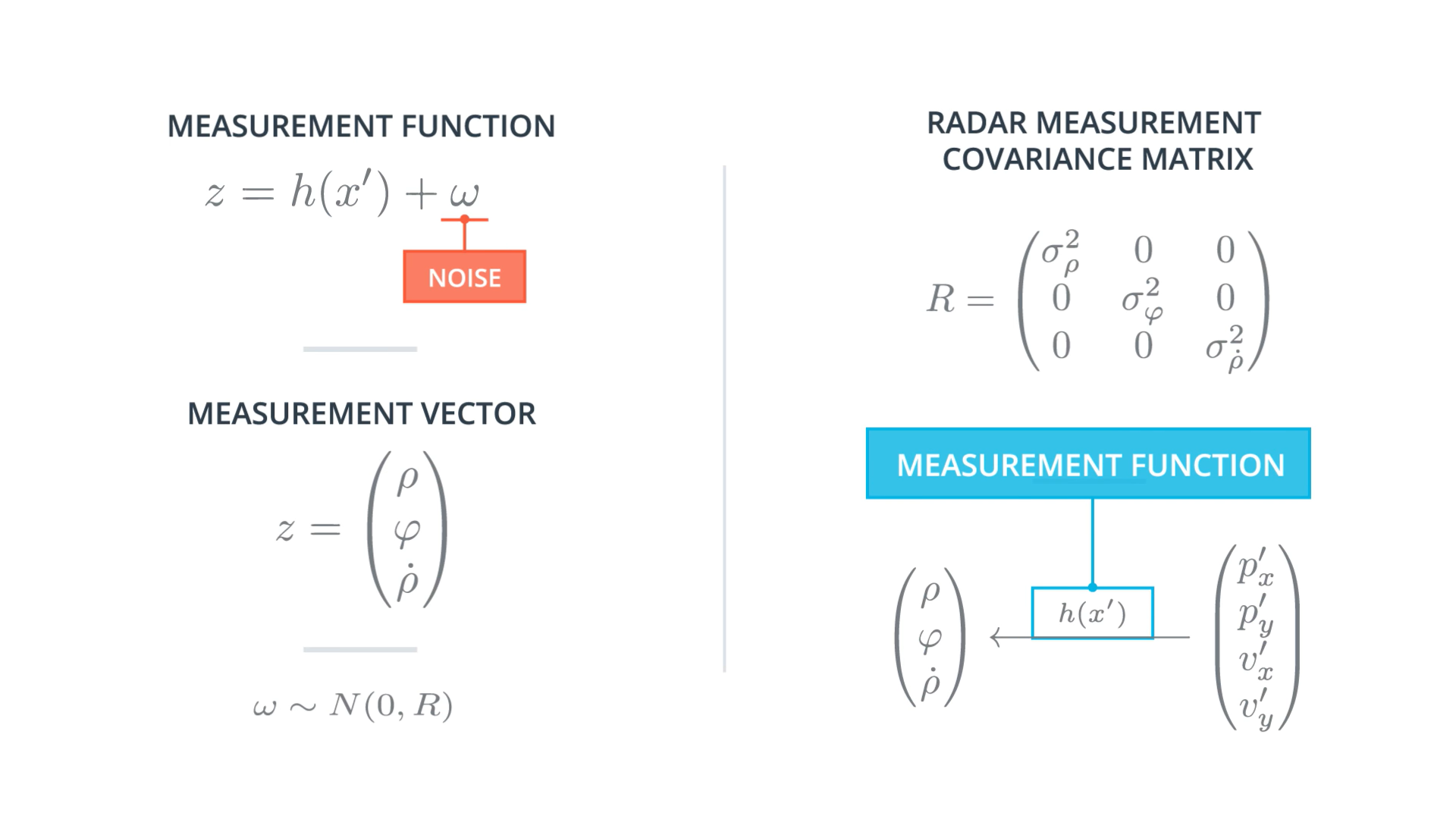
- Considering that the three measurement vector components are not cross correlated, the Radar measurement covariance matrix becomes 3x3 diagonal matrix.
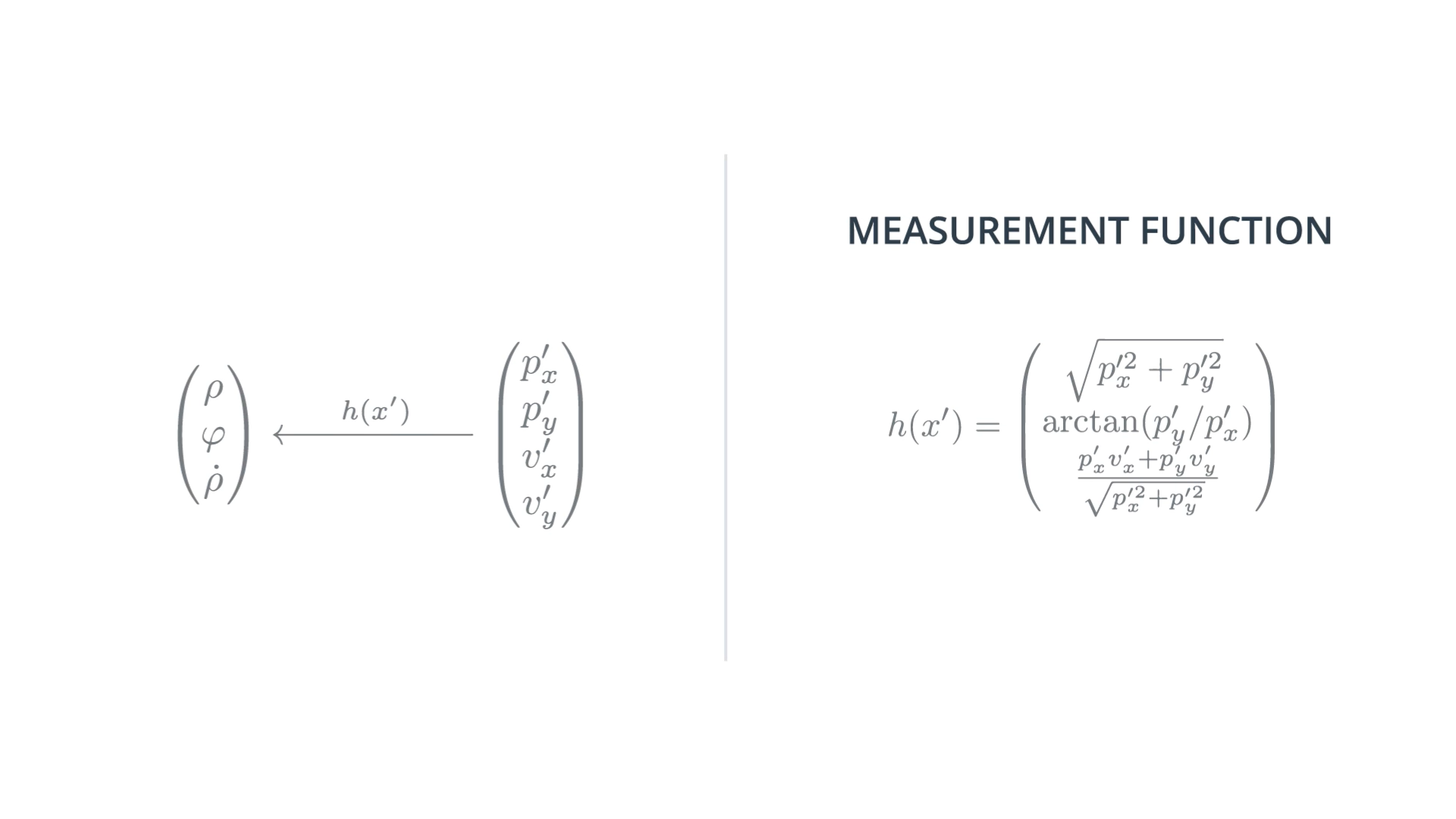
H versus h(x)
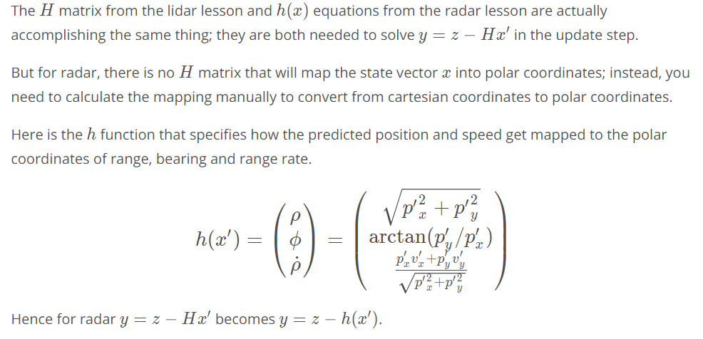
Definition of Radar Variables

Deriving the Radar Measurement Function
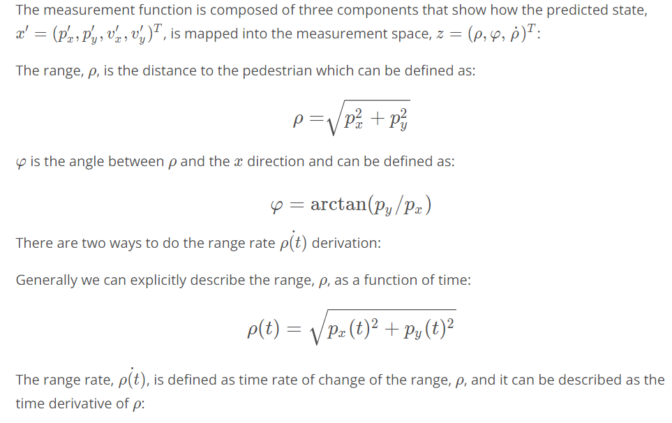
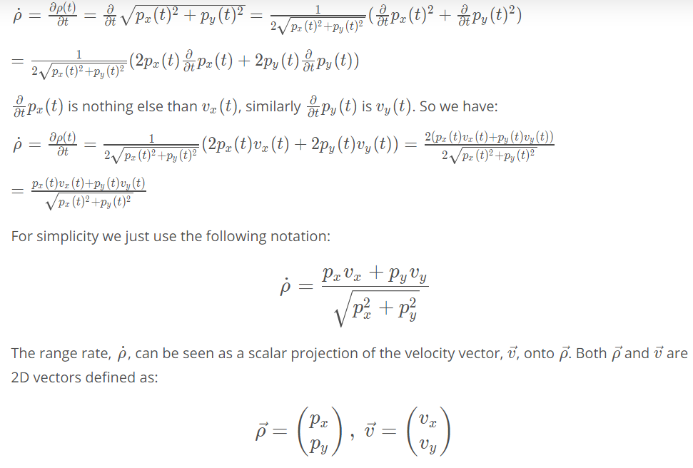

Question?
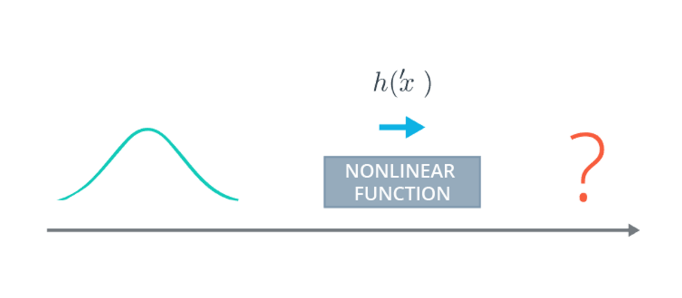
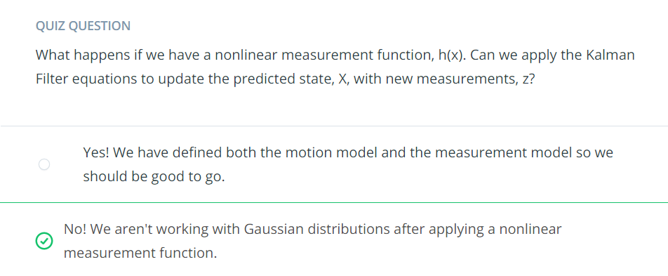
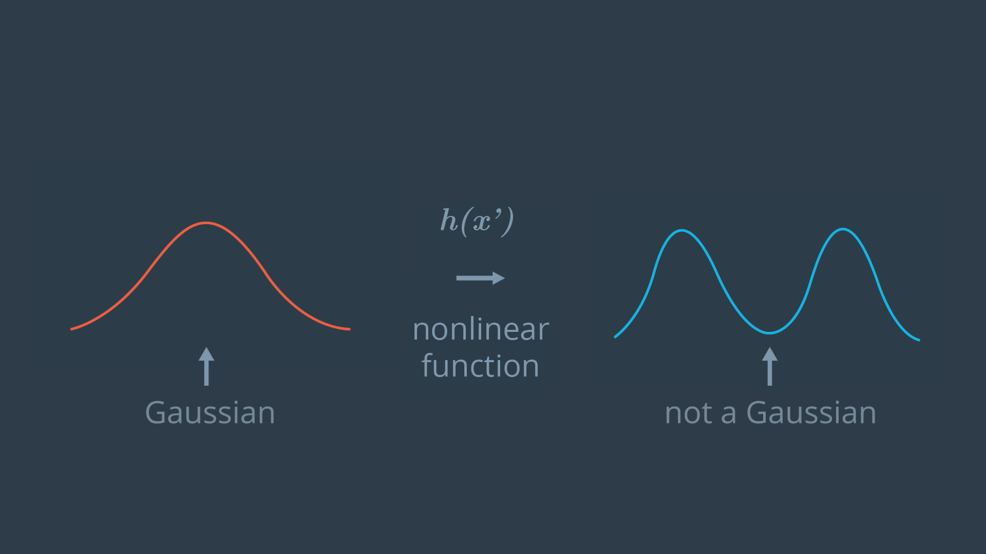
So the Kalman filter update equations is not applicable anymore.
Extended Kalman Filter
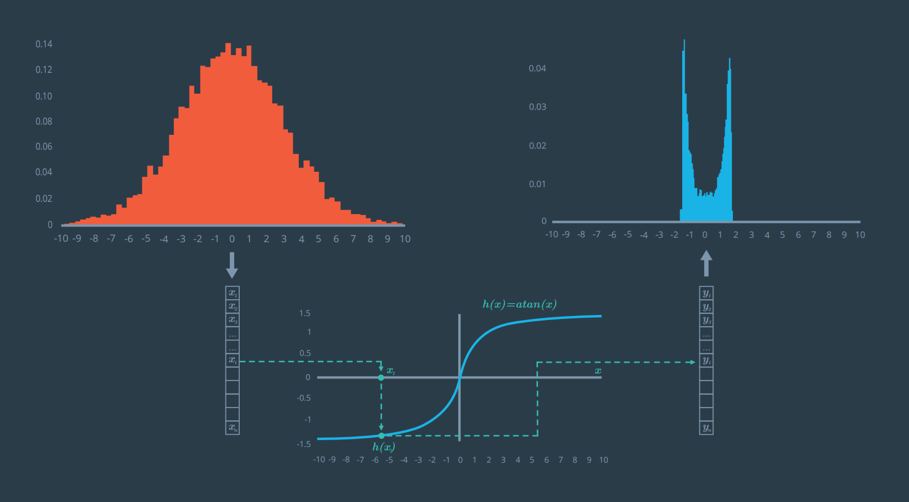
A possible solution is to linearize the h(x) function, and that is the key idea of EKF.
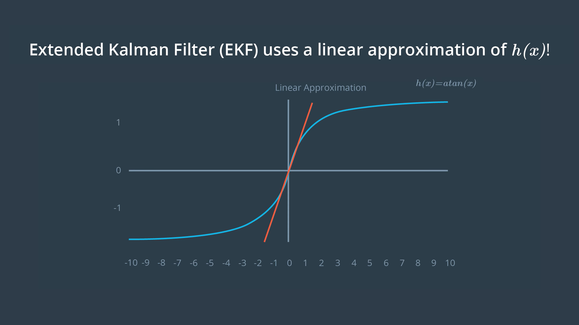
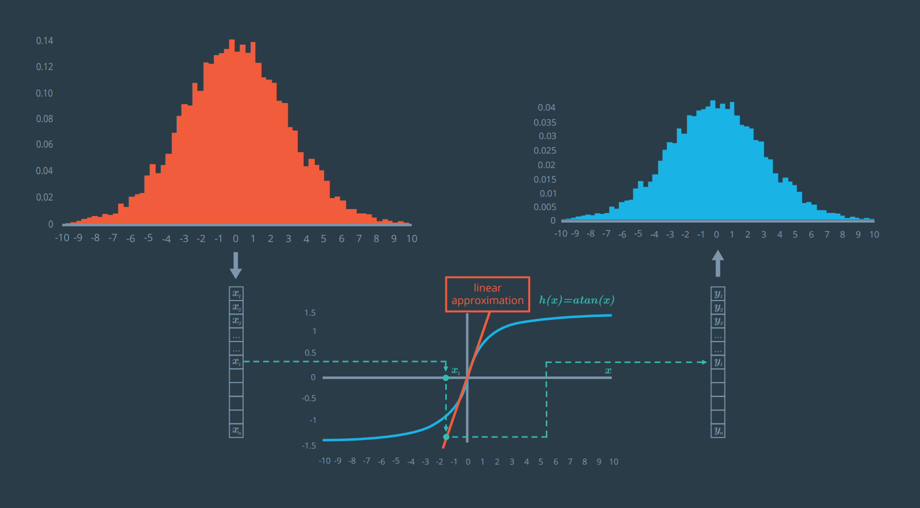
How to Perform a Taylor Expansion
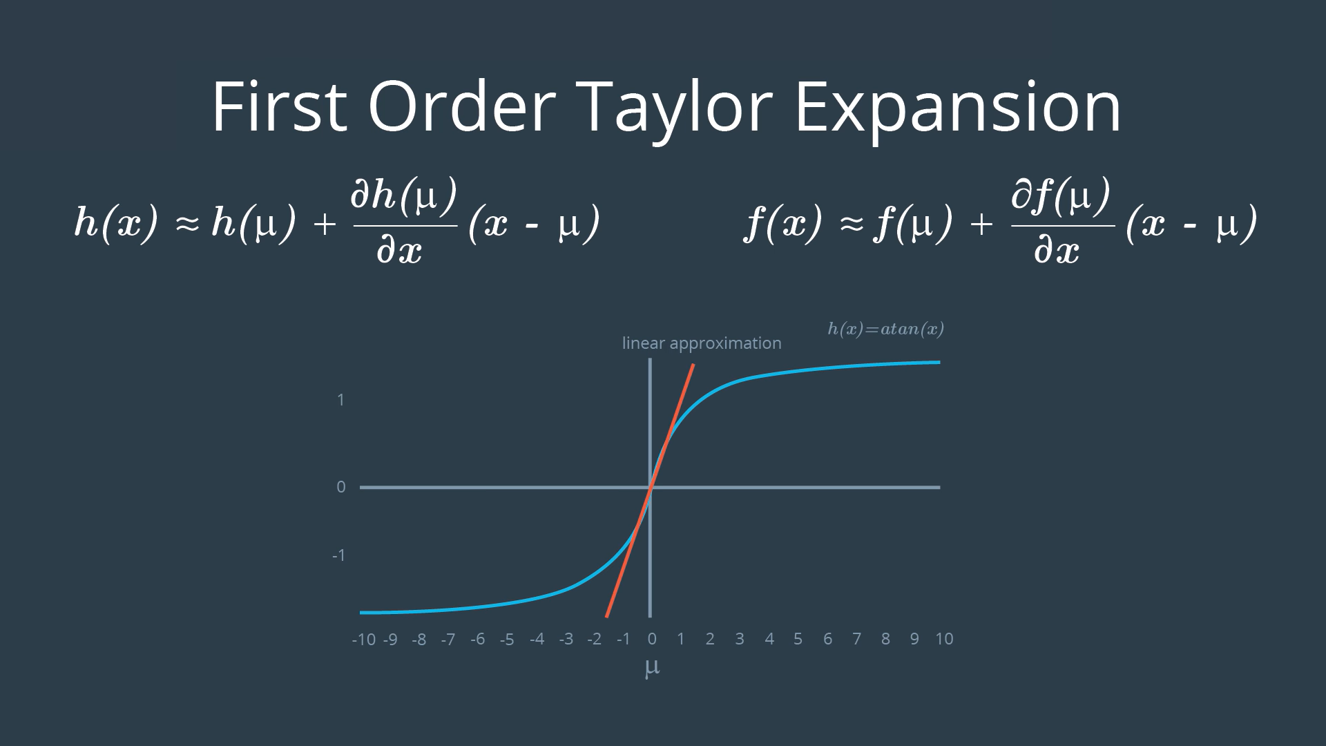
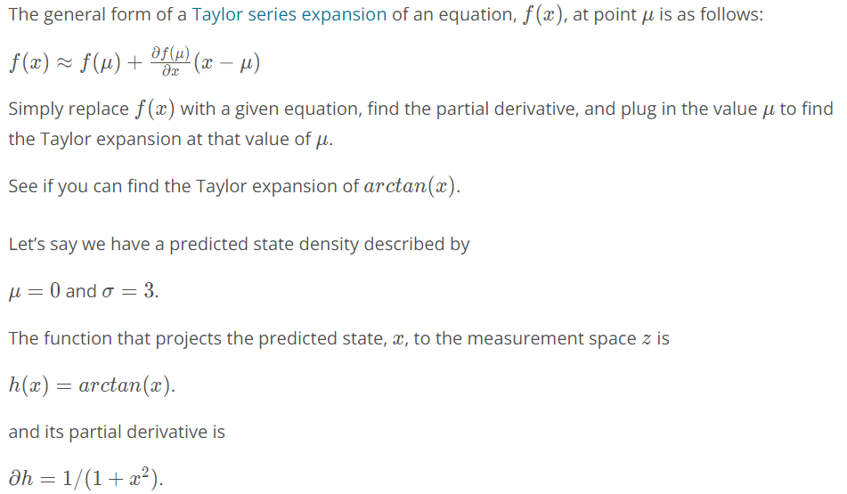
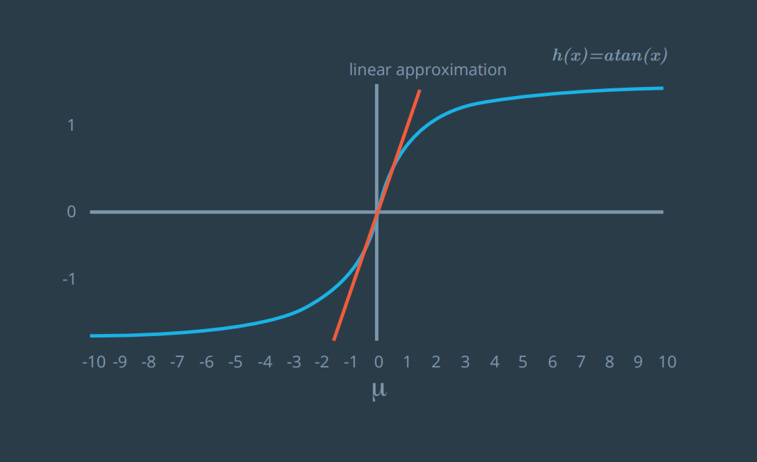

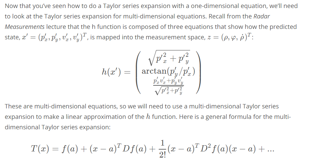
Multivariate Taylor Series


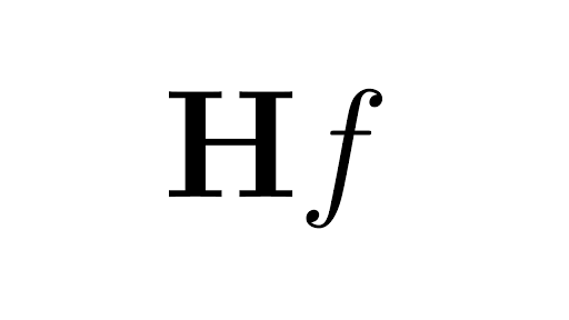
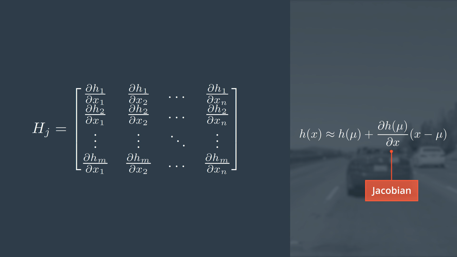
Jacobian Matrix
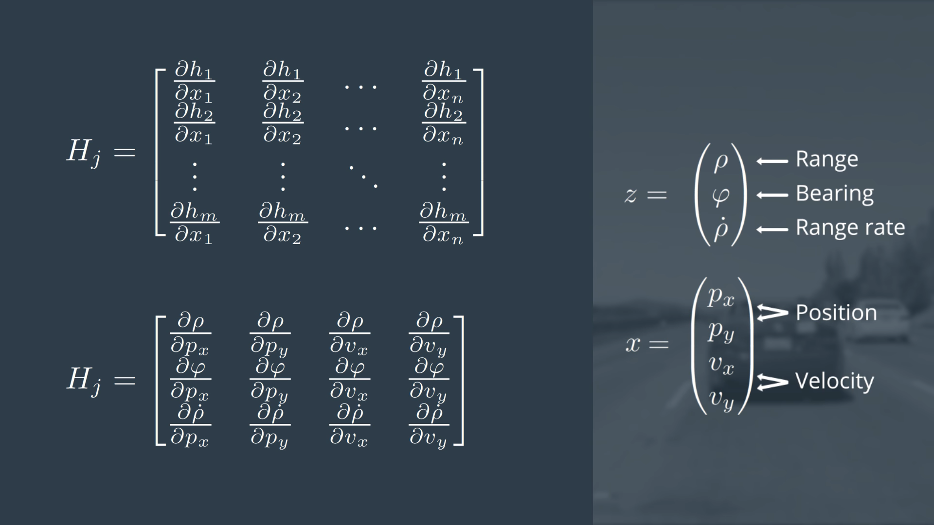
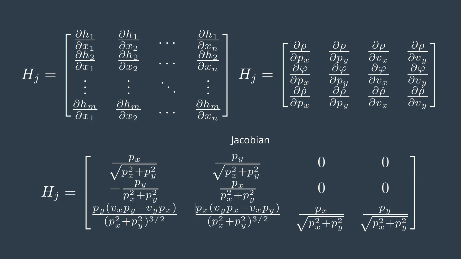
EKF Algorithm Generalization
Extended Kalman Filter Equations


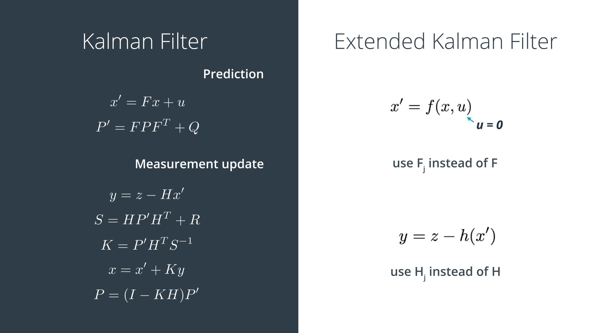
Clarification of u = 0

More Details About Calculations with Radar Versus Lidar
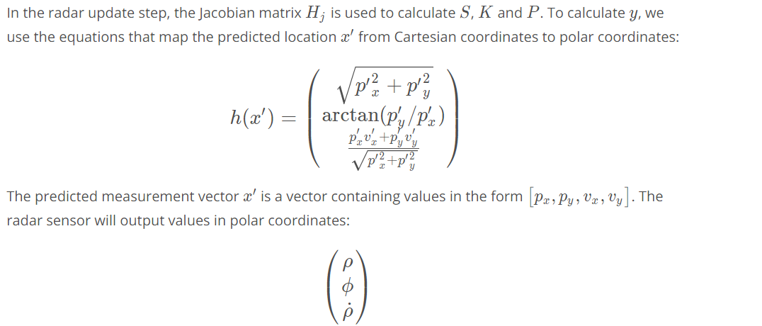
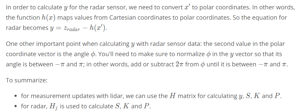
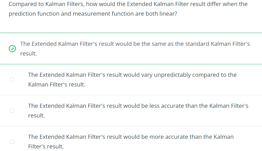
If f and h are linear functions, then the Extended Kalman Filter generates exactly the same result as the standard Kalman Filter. Actually, if f and h are linear then the Extended Kalman Filter F_j turns into f and H_j turns into h. All that's left is the same standard Kalman Filter!
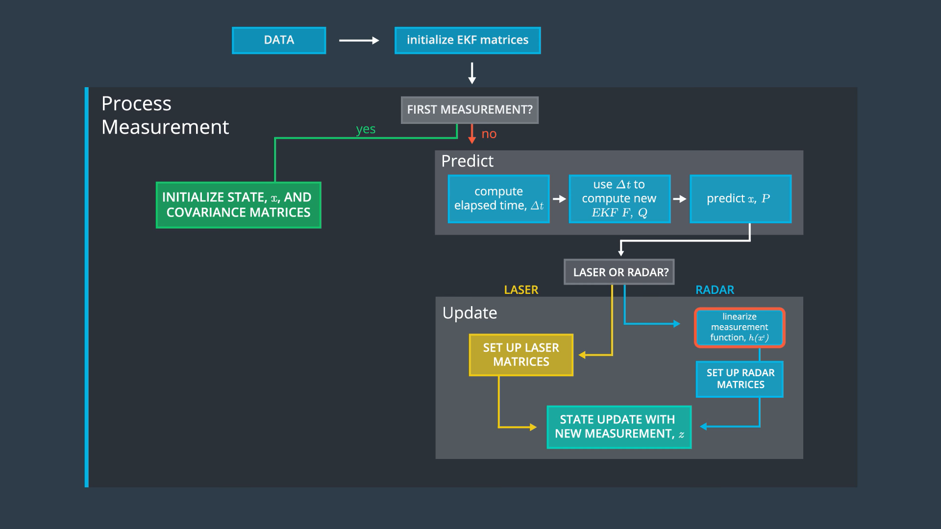
In our case we have a linear motion model, but a nonlinear measurement model when we use radar observations. So, we have to compute the Jacobian only for the measurement function.
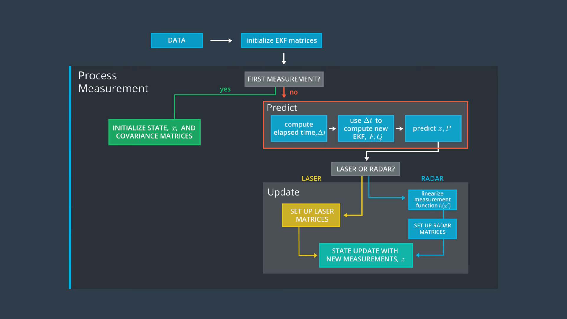
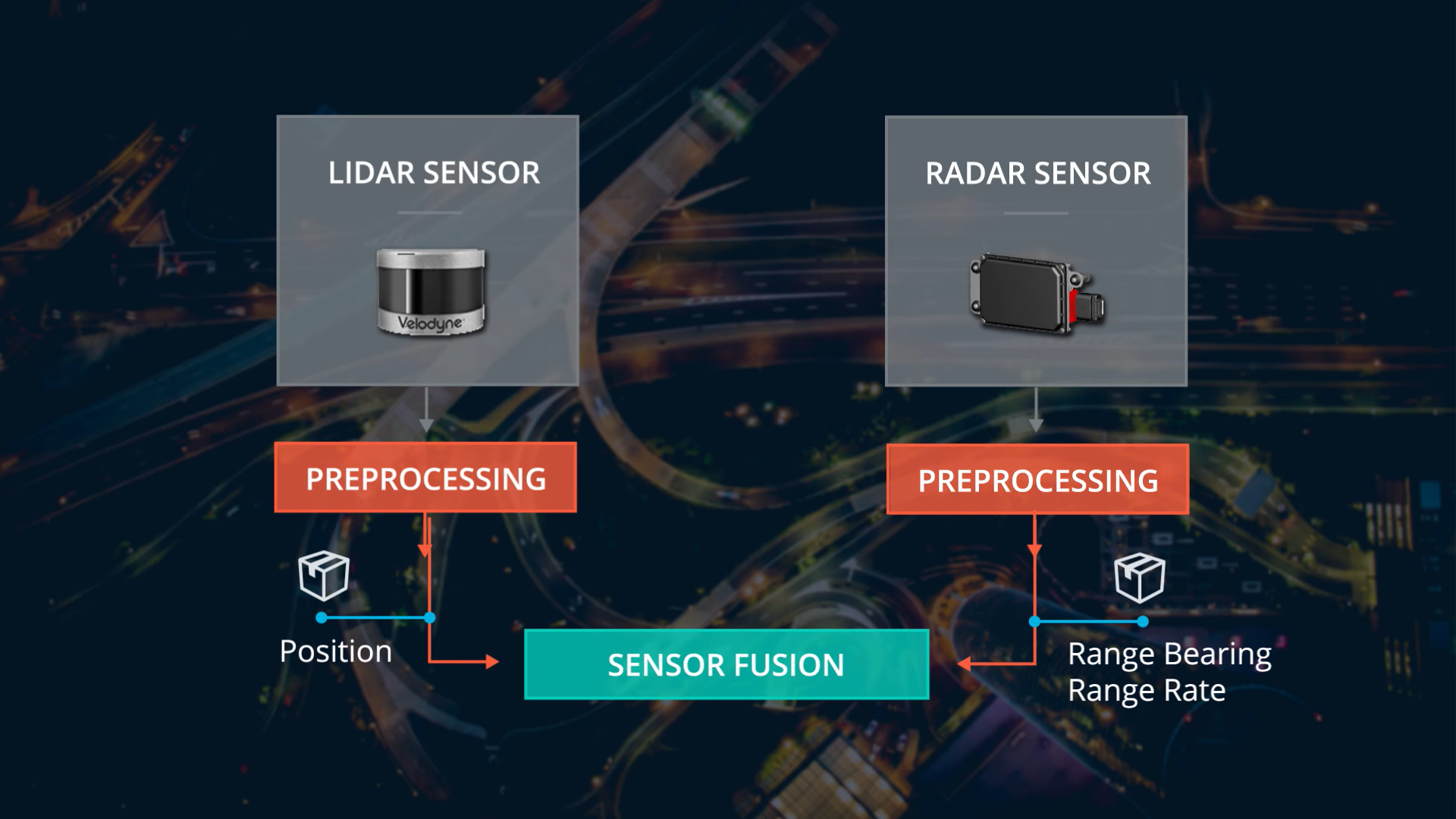
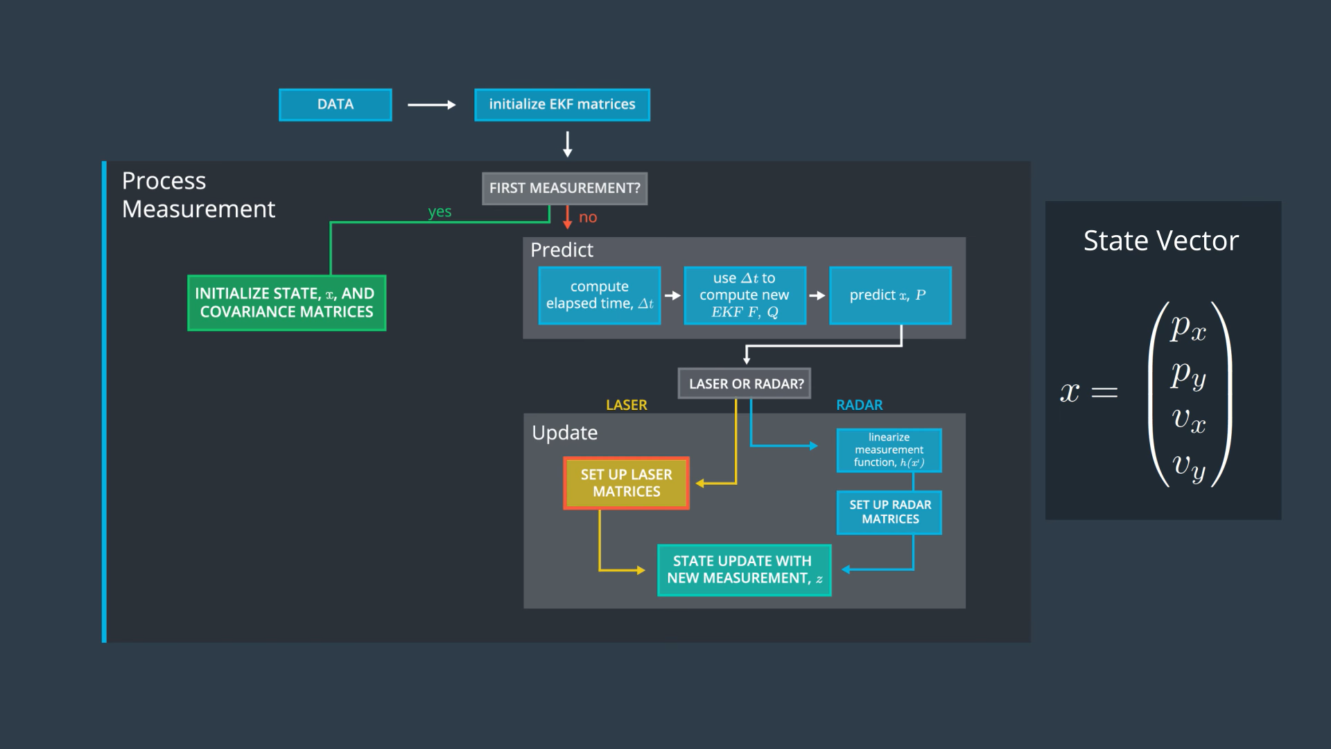
Sensor Fusion General Flow
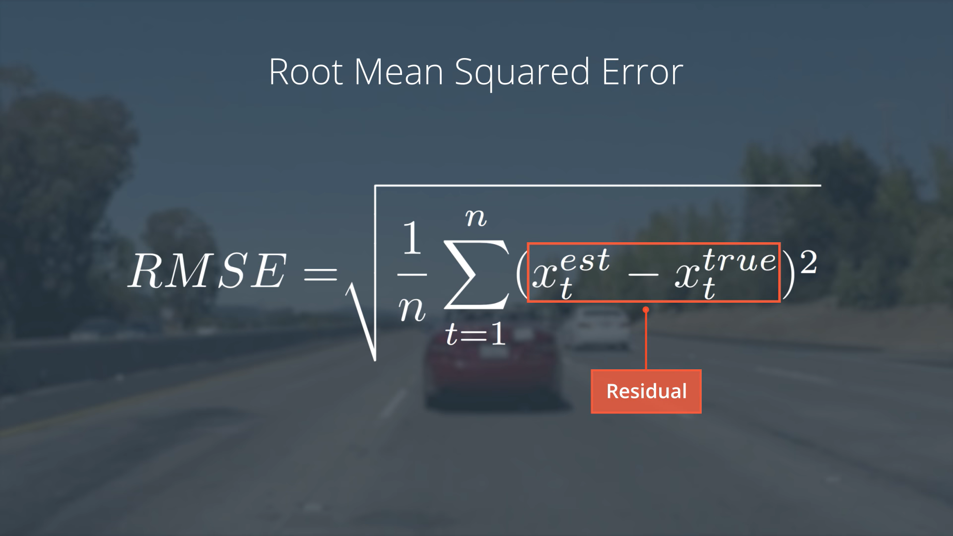
Evaluating KF Performance
