Descriptor Matching

Once you have located and described a set of keypoints for each image in a sequence of frames, the next step in the tracking process is to find the best fit for each keypoint in successive frames. In order to do so, you need to implement a suitable similarity measure so that your tracking algorithm can uniquely assign keypoint pairs.

You will learn how to properly deal with ambiguities that can occur when features look very similar. The section will conclude with an overview of performance measures (e.g. true positive rate) to describe the quality of a matching method so you will be able to compare algorithms and make an informed choice when it comes down to selecting a suitable method for your project.

We focus on three main aspects:

1. Similarity measures - How to gauge the similarity between two descriptors?

2. Where to position the selection threshold? and what about unwanted correspondences? How to decide whether two descriptors are similar based on similarity measure? Main question is:

3. Overview of methods and concepts for accessing the performance of detectors and descriptors to find out which one is suited for our particular problem.

Distance between descriptors

In the last section, you have learned that keypoints can be described by transforming their local neighborhood into a high-dimensional vector that captures the unique characteristics of the gradient or intensity distribution. In this section, we want to look at several ways to compute the distance between two descriptors such that the differences between them are transformed into a single number which we can use as a simple measure of similarity.

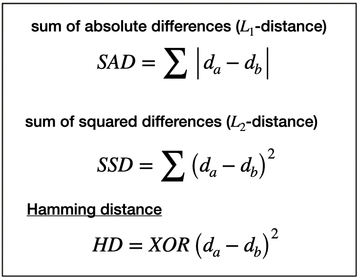
The first distance function is the "Sum of Absolute Differences (SAD)". As you can see in the equation below, the SAD takes as input two descriptor vectors d_ada and d_bdb. The SAD is computed by subtracting from every component in d_ada the corresponding component at the same position in d_bdb. Then, the absolute value of the respective result is summed up. The SAD norm is also referred to as L1-norm in the literature.

The second distance function is the "Sum of Squared Differences (SSD)", which is similar to the SAD in the sense that differences between individual components of two descriptor vectors are computed. However, the key difference between SAD and SSD is that the latter sums the squared differences instead of the absolute differences. In the literature, the SSD norm is also referred to as L2-norm. Both norms are given in the following figure.

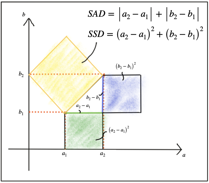
There are several ways of explaining the differences between SAD and SSD. One helpful approach, as we want to keep this aspect short, is to look at both norms from a geometrical perspective. In the following figure, a two-dimensional feature space is considered. In it, there are two feature vectors d1 and d2, each of which consists of an (a,b) coordinate pair.

The shortest distance between both is a straight line. Given the two components of each vector, the SAD computes the sum of the length differences, which is a one-dimensional process. The SSD on the other hand, computes the sum of squares, which obeys the law of Pythagoras. This law says that in a rectangular triangle, the sum of the catheti squares is equal to the square of the hypotenuse. So in terms of the geometric distance between both vectors, the L2-norm is a more accurate measure. Note that the same rationale applies to higher-dimensional descriptors in the same manner.

In the case of a binary descriptor who consists only of ones and zeros, the best (and fastest) measure to use is the Hamming distance, which computes the difference between both vectors by using an XOR function, which returns zero if two bits are identical and one if two bits are different. So the sum of all XOR operations is simply the number of differing bits between both descriptors.

The key takeaway here is that you have to adapt the distance measure to the type of descriptor you are using. In case of gradient-based methods such as SIFT, the L2-norm would be most appropriate. In the case of all binary descriptors, the Hamming distance should be used.

Finding matches

Let us assume we have N keypoints and their associated descriptors in one image and M keypoints in another image. The most obvious method to look for corresponding pairs would be to compare all features with each other, i.e. perform N x M comparisons. For a given keypoint from the first image, it takes every keypoint in the second image and calculates the distance. The keypoint with the smallest distance will be considered its pair. This approach is referred to as Brute Force Matching or Nearest Neighbor Matching and is available in the OpenCV under the name BFMatcher. The output of brute force matching in OpenCV is a list of keypoint pairs sorted by the distance of their descriptors under the chosen distance function. Brute force matching works well for small keypoint numbers but can be computationally expensive as the number of keypoints increases.

In 2014, David Lowe (the father of SIFT) and Marius Muja released an open-source library called "fast library for approximate nearest neighbors" (FLANN). FLANN trains an indexing structure for walking through potential matching candidates that is created using concepts from machine learning. The library builds a very efficient data structure (a KD-tree) to search for matching pairs and avoids the exhaustive search of the brute force approach. It is therefore faster while the results are still very good, depending on the matching parameters. As FLANN-based matching entails a whole new body of knowledge with several concepts that have limited relevance for this course, there is no detailed description of the method given here. The FLANN-based matching is available in the OpenCV and you will see it again in the code example below. At the time of writing (May 2019), there is a potential bug in the current implementation of the OpenCV, which requires a conversion of the binary descriptors into floating point vectors, which is inefficient. Yet still there is an improvement in speed, albeit not as large as it potentially could be.

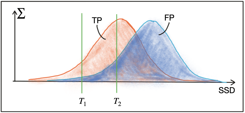
Both BFMatching and FLANN accept a descriptor distance threshold T which is used to limit the number of matches to the ‘good’ ones and discard matches where the respective pairs are no correspondences. Corresponding ‘good’ pairs are termed ‘True Positives (TP)’ whereas mismatches are called ‘False Positives (FP)’. The task of selecting a suitable value for T is to allow for as many TP matches as possible while FP matches should be avoided as far as possible. Depending on the image content and on the respective detector / descriptor combination, a trade-off between TP and FP has to be found that reasonably balances the ratio between TP and FP. The following figure shows two distributions of TP and of FP over the SSD to illustrate threshold selection.

The first threshold T1 is set to a maximally permissible SSD between two features in a way that some true positive matches are selected, while false positive matches are almost entirely avoided . However, most TP matches are also discarded with this setting. By increasing the matching threshold to T2, more TP matches are selected but the number of FP matches also increases significantly. In practice, a clear and concise separation of TP and FP is almost never found and therefore, setting a matching threshold is always a compromise between balancing 'good' vs. 'bad' matches. While FP matches can not be avoided in most cases, the goal always is to lower their number as much as possible. In the following, two strategies to achieve this are presented.

Selecting Matches

As long as the selected threshold T is not exceeded, brute force matching will always return a match for a keypoint in the first image, even if the keypoint is not present in the second image. This inevitably leads to a number of false matches. A strategy to counteract this is called cross check matching, which works by applying the matching procedure in both directions and keeping only those matches whose best match in one direction equals the best match in the other direction. The steps of the cross check approach are:

1. For each descriptor in the source image, find one or more best matches in the reference image.

2. Switch the order of source and reference image.

3. Repeat the matching procedure between source and reference image from step 1.

4. Select those keypoint pairs whose descriptors are best matches in both directions.

Although cross check matching increases the processing time, it usually removes a significant number of false matches and should thus always be performed when accuracy is preferred over speed.

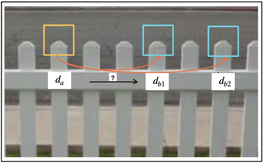
A very efficient way of lowering the number of false positives is to compute the nearest neighbor distance ratio for each keypoint. This method has been originally proposed by D. Lowe in the 1999 paper on SIFT. The main idea is to not apply the threshold on the SSD directly. Instead, for each keypoint in the source image, the two best matches are located in the reference image and the ratio between the descriptor distances is computed. Then, a threshold is applied to the ratio to sort out ambiguous matches. The figure below illustrates the principle.

In the example, an image patch with an associated descriptor da is compared to two other image patches with descriptors db1 and db2. As can be seen, the patches look very similar and would result in ambiguous and thus unreliable matches. By computing the SSD ratio between best and second-best match, such weak candidates can be filtered out.

In practice, a threshold value of 0.8 has proven to provide a good balance between TP and FP. In the image sequences examined in the original SIFT paper, 90% of the false matches were eliminated with this setting while less than 5% of correct matches were lost.

Tracking an Object Across Images

How to track an object across multiple camera images and verify it is the same object?

You definitely have to have a central track management system. If you don't have overlap between sensors, then you have some blind spot. You can also predict your object throughout occlusions for a little bit. That is OK, but if the gap is too large or the object is occluded for a longer period of time, then there will be an ID switch and the planner has to properly react to that.

Should camera images be treated as related to each other or as individual images?

Consecutive camera images are extremely correlated and that is a good thing. If you want to correspondences between consecutive images, you make use of the fact that they are so correlated. You can find many correspondences and compute optical flow which allow you to do many great things.

Optical flow

Optical flow is 2D vector field, the displacement of every pixel in the previous frame to a pixel in the current frame. If you have those correspondences, you can do things like structure from motion, visual odometry and object tracking.

Structure from motion

It is the process of inferring depth by moving through a scene. You can reconstruct the 3D environment by either stereo, or by structure from motion. In stereo, you have two images taken at the same time, and there is a difference between the 2 images' positions. In structure from motion, you take two consecutive images by the same camera, so the displacement is basically the distance you traveled. The great thing about that you can extract that from mono camera, but only as long as you are moving. That's one of the downsides of structure from motion.