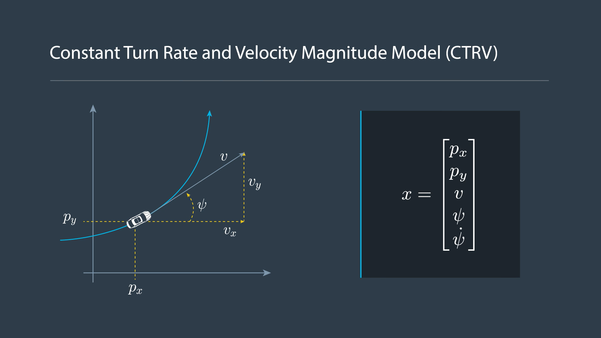
The CTRV Model

Motion Models and Kalman Filters

In the extended kalman filter lesson, we used a constant velocity model (CV). A constant velocity model is one of the most basic motion models used with object tracking.

But there are many other models including:

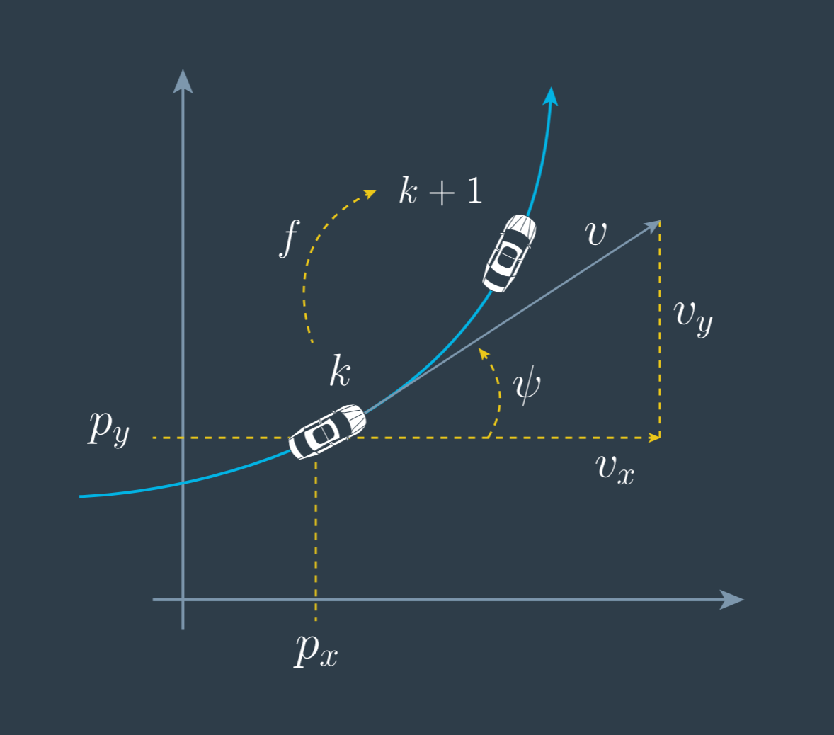
• constant turn rate and velocity magnitude model (CTRV)

• constant turn rate and acceleration (CTRA)

• constant steering angle and velocity (CSAV)

• constant curvature and acceleration (CCA)

Each model makes different assumptions about an object's motion. In this lesson, you will work with the CTRV model.

Keep in mind that you can use any of these motion models with either the extended Kalman filter or the unscented Kalman filter, but we wanted to expose you to more than one motion model.

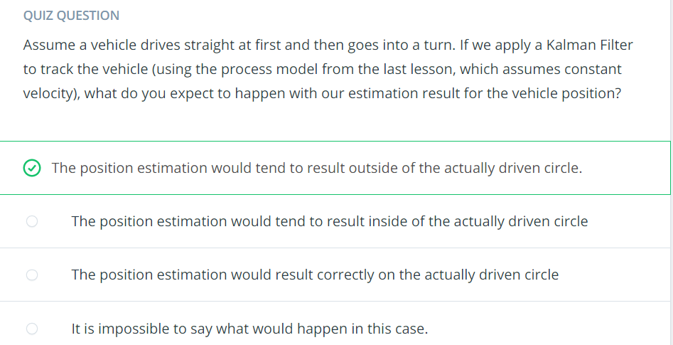
Right! The process model would assume the car is moving tangentially to the circle, resulting in a predicted position outside of it.

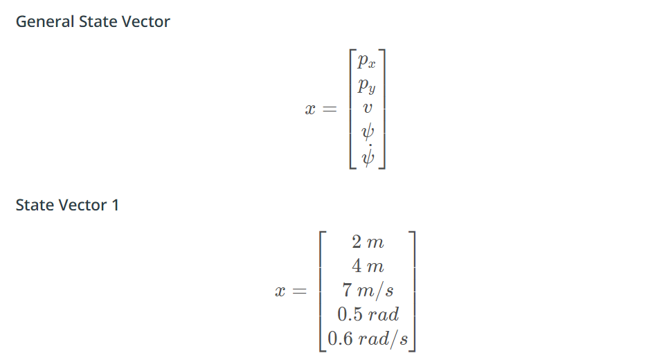
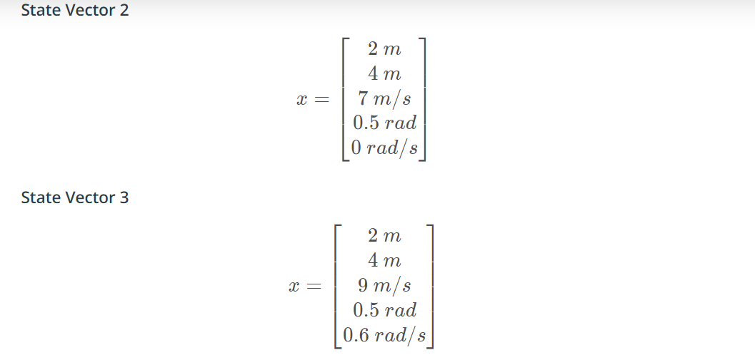
Right! Though 1 and 3 have the same yaw rate, state vector 1 has a slower speed, meaning the car would make a complete circle in less distance.

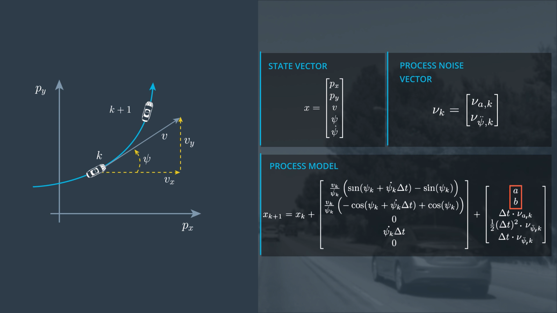
CTRV Differential Equation

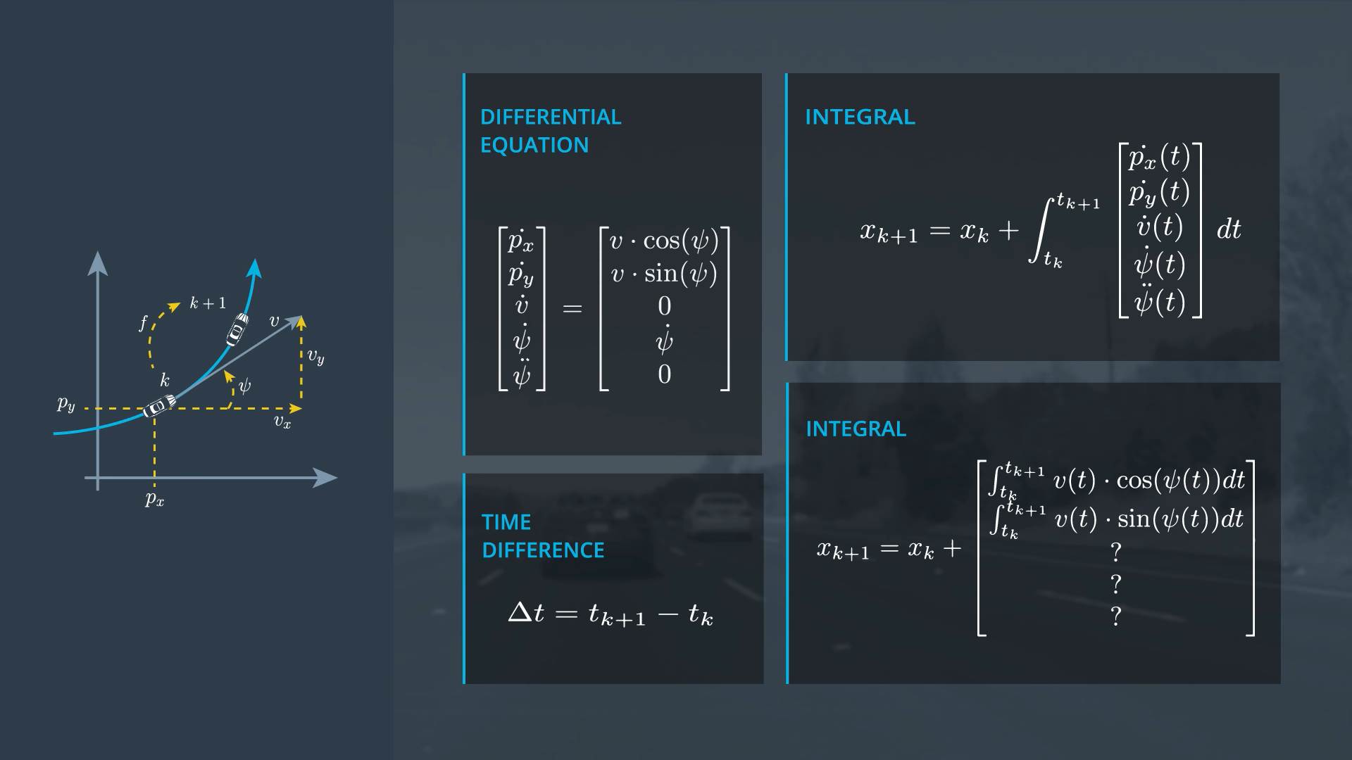
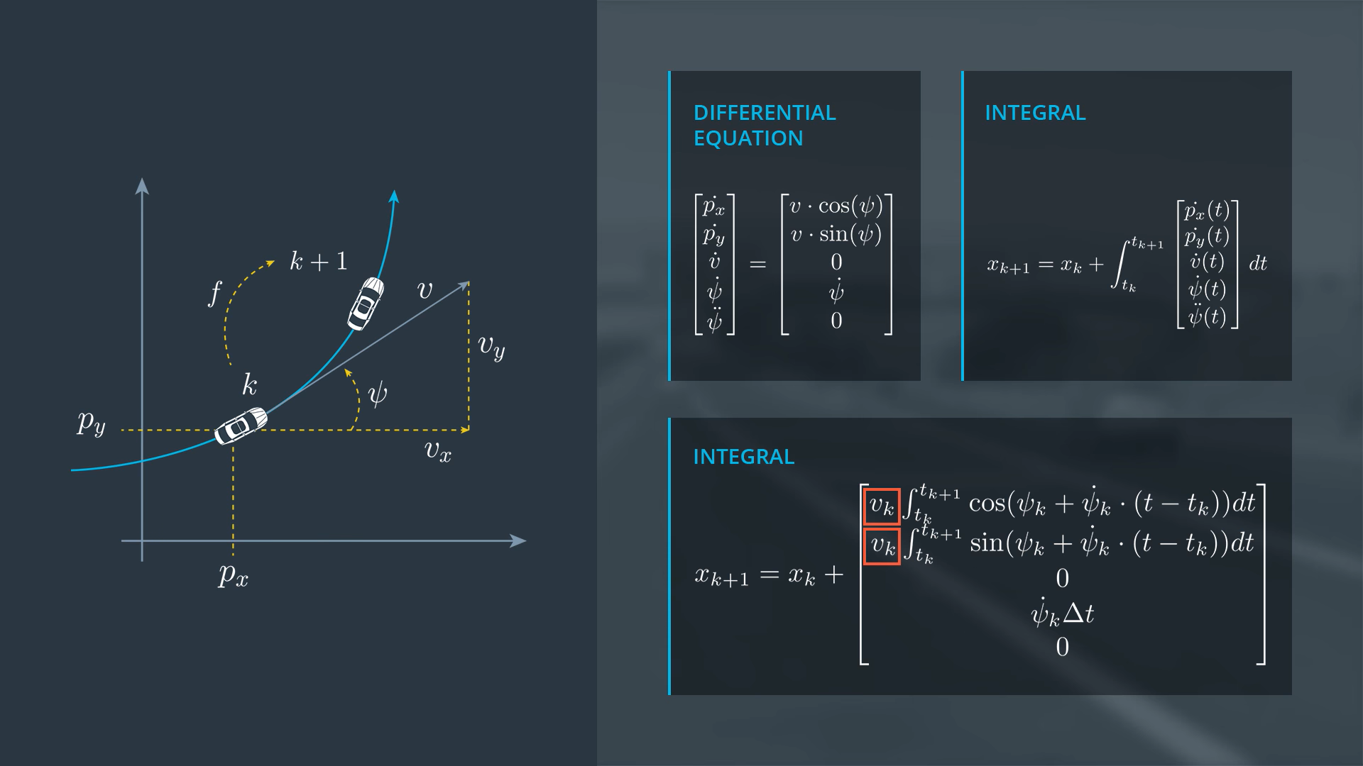
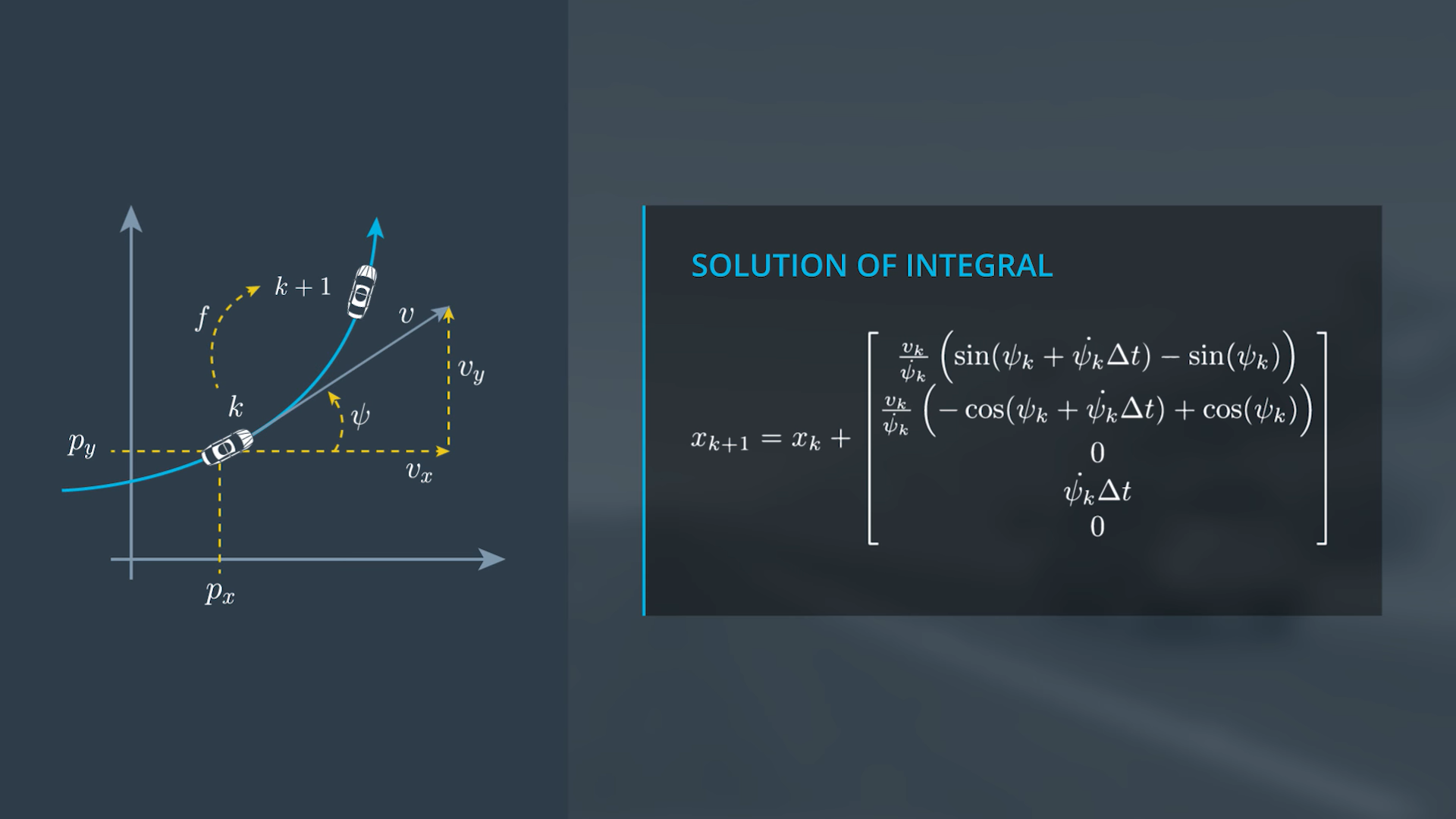
CTRV Zero Yaw Rate

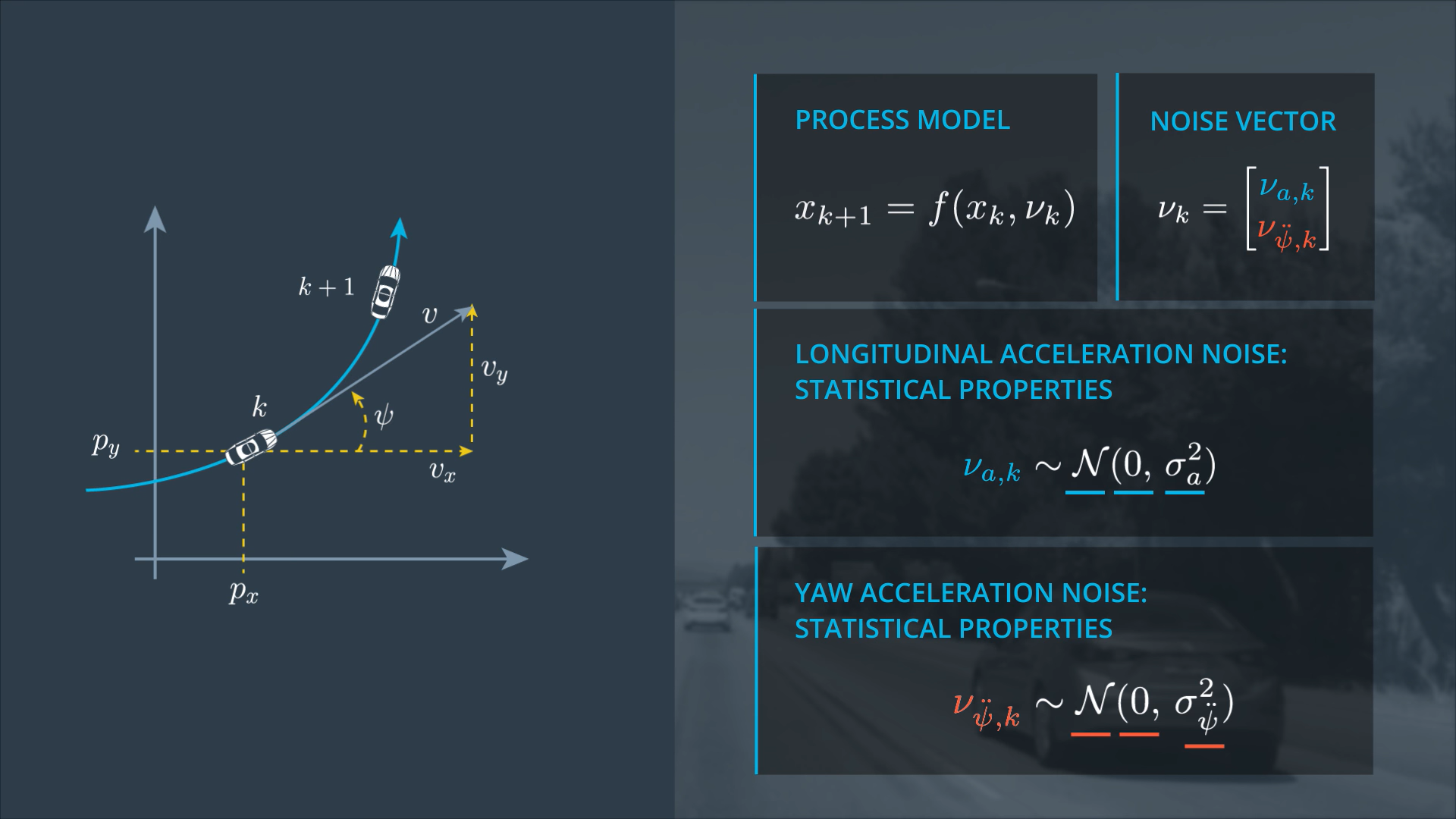
CTRV Process Noise Vector

UKF Process Chain

Unscented Kalman Filter Introduction

Now that you have learned the CTRV motion model equations, we will discuss how the unscented Kalman filter works. As you go through the lectures, recall that the extended Kalman filter uses the Jacobian matrix to linearize non-linear functions.

The unscented Kalman filter, on the other hand, does not need to linearize non-linear functions; instead, the unscented Kalman filter takes representative points from a Gaussian distribution. These points will be plugged into the non-linear equations as you'll see in the lectures.

What Problem Does the UKF Solve?

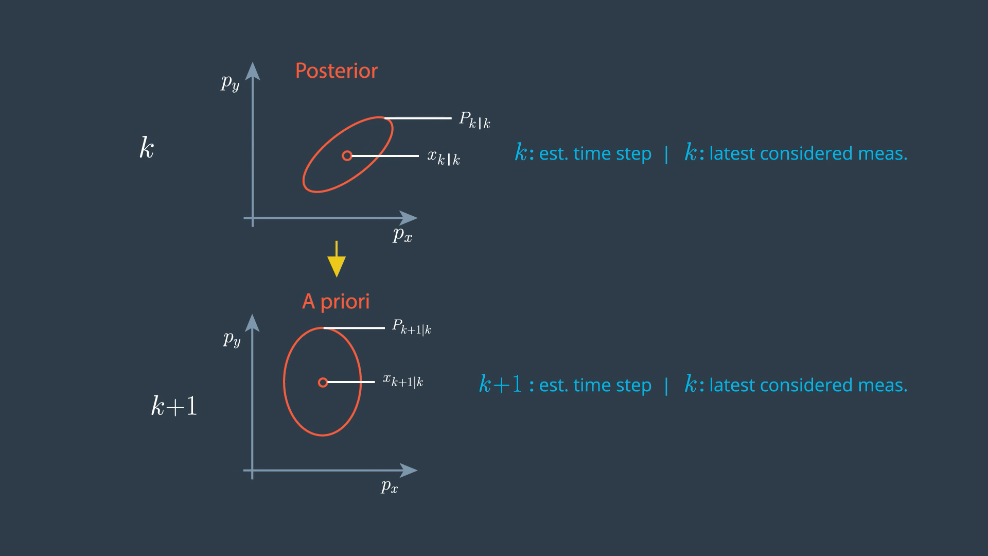
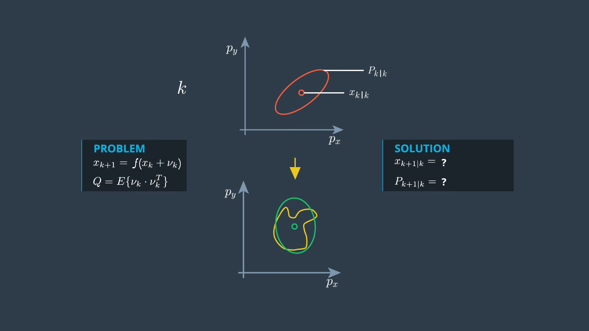
• These ellipses describe the distribution of our uncertainty, all points on this line have the same probability density. If the uncertainty is normally distributed, these points have the shape of an ellipse. It can be seen as the visualization of the covariance matrix P.

→ If the process model is linear, the prediction problem looks like this:

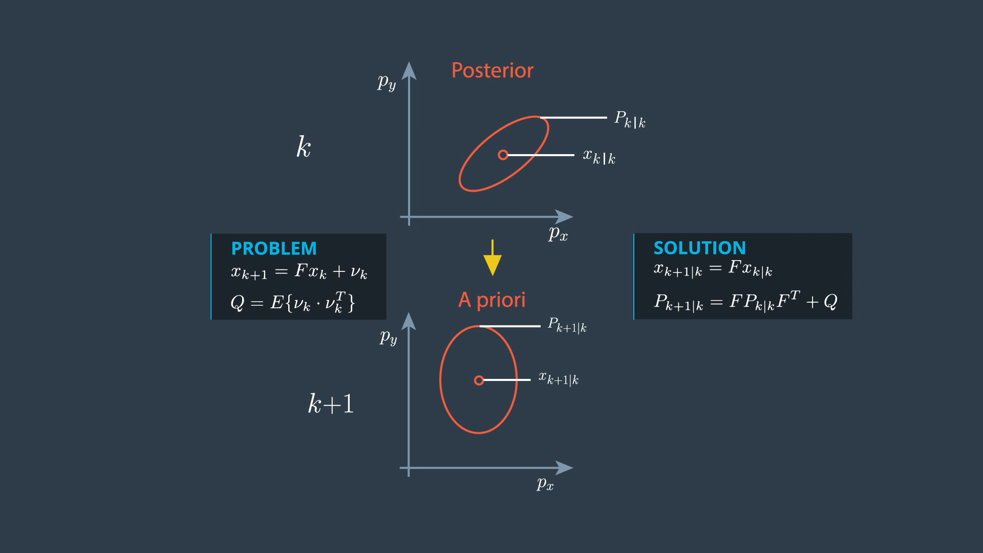
→ Q is the covariance matrix of the process noise. We can use Kalman filter so solution is linear prediction problem.

• If the process model is non linear, then the prediction is defined by non-linear function f. Predicting with non-linear function provides a distribution which is generally not linearly distributed any more. This distribution can only be calculated numerically (yellow distribution). We want to find the normal distribution that represents the real predicted distribution as close as possible. In other words, we look for the normal distribution which has the same mean and the same covariance matrix as the real predicted distribution (green distribution). This is what the unscented transformation does for us.

UKF Basics Unscented Transformation

It can be difficult to transform the whole state distribution through non linear function, but it is very easy to transform the individual points of the state space through the non linear function. This is what Sigma points are for. The Sigma points are chosen around the mean state and in a certain relation to the standard deviation sigma of every state dimension (this is why these points are called sigma points). They serve as a representative of the whole distribution.

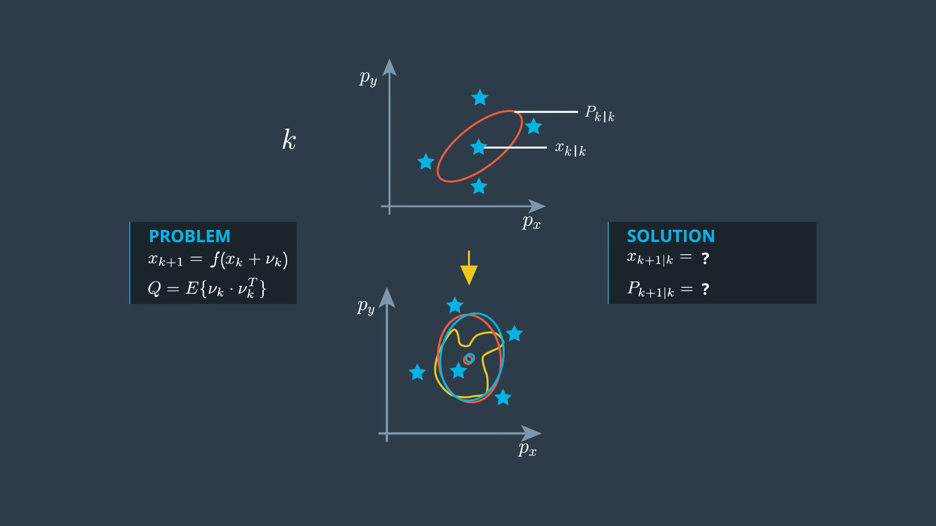
Once you have chosen the sigma points, you just insert every single sigma point into the non linear function f → so they come somewhere in the predicted space. All you have to do now is calculate the mean and covariance of the group of sigma points. This will not provide the same mean and covariance of the predicted distribution but it gives useful approximation.

If the process model is linear, the Sigma points approach provides exactly the same solution as the standard Kalman filter (but they are more expensive in terms of calculation time).

We Can Split the Prediction Step into 3 Parts

1. A good way to choose the sigma points

2. How to predict the sigma points → Just insert them into the process function

3. Calculate the prediction mean and covariance from the predicted sigma points

Step 1: Generating Sigma Points

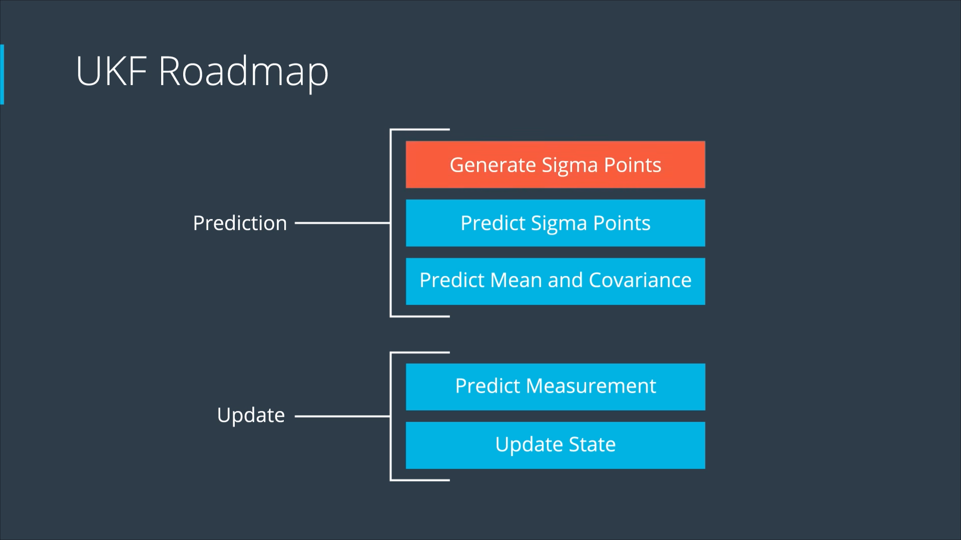
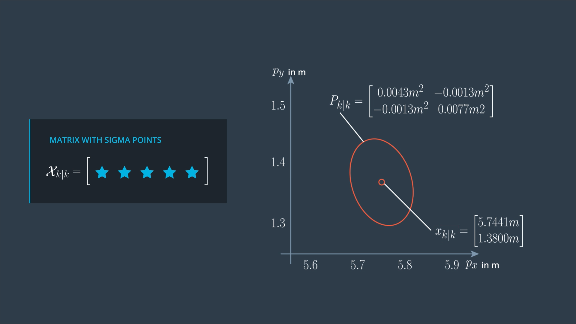
At the beginning of the prediction step, we have the posterior state Xk|k, and the posterior covariance matrix Pk|k from the last iteration. These represent the distribution of our current state. For this distribution, we want to generate sigma points.

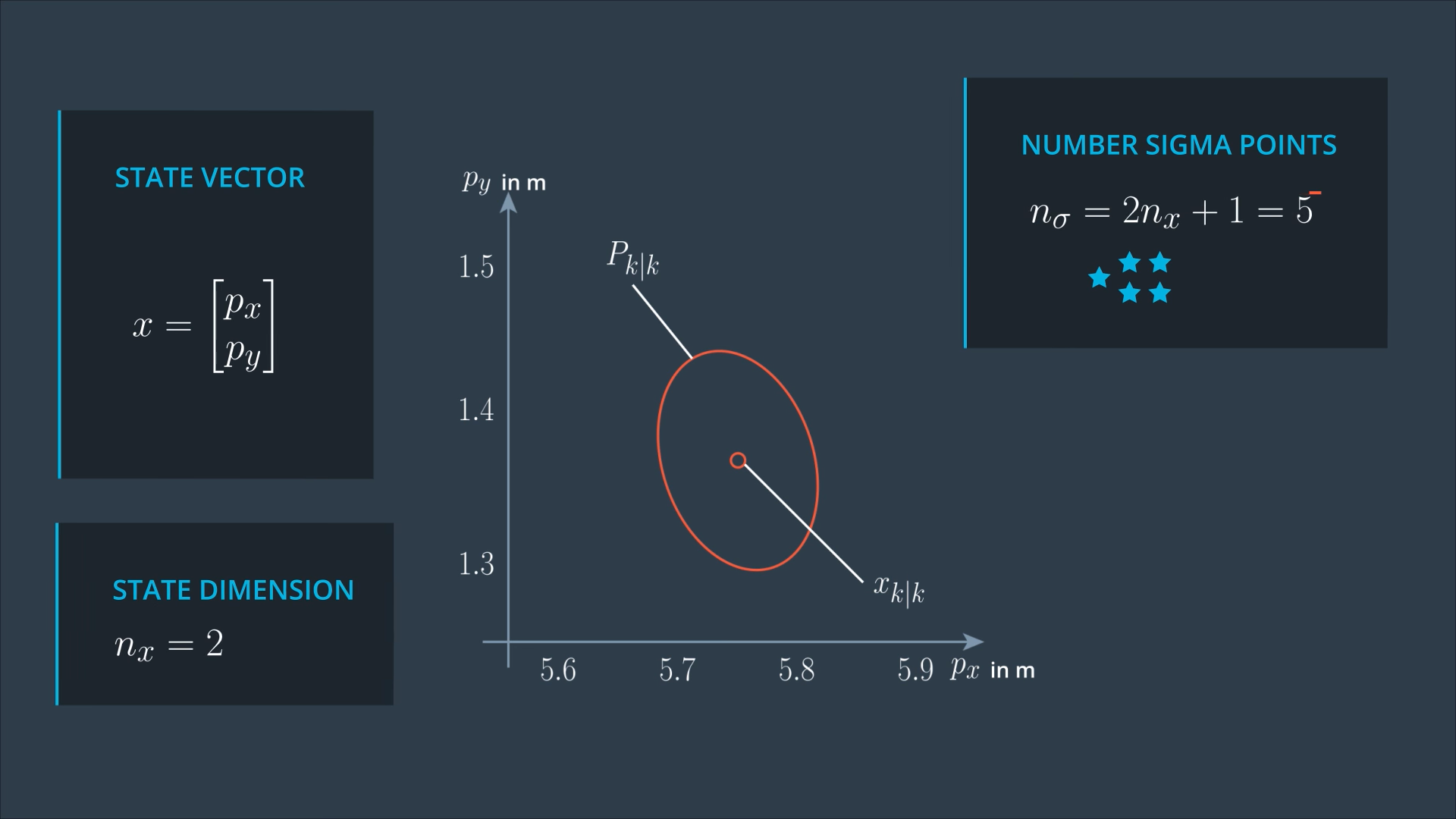
The number of sigma points depends on the state dimension, since we are dealing with CTRV model, so the dimension of our state is 5.

The first sigma point is the mean of the state, then we have 2 points per state dimension, which will be spread in different directions.

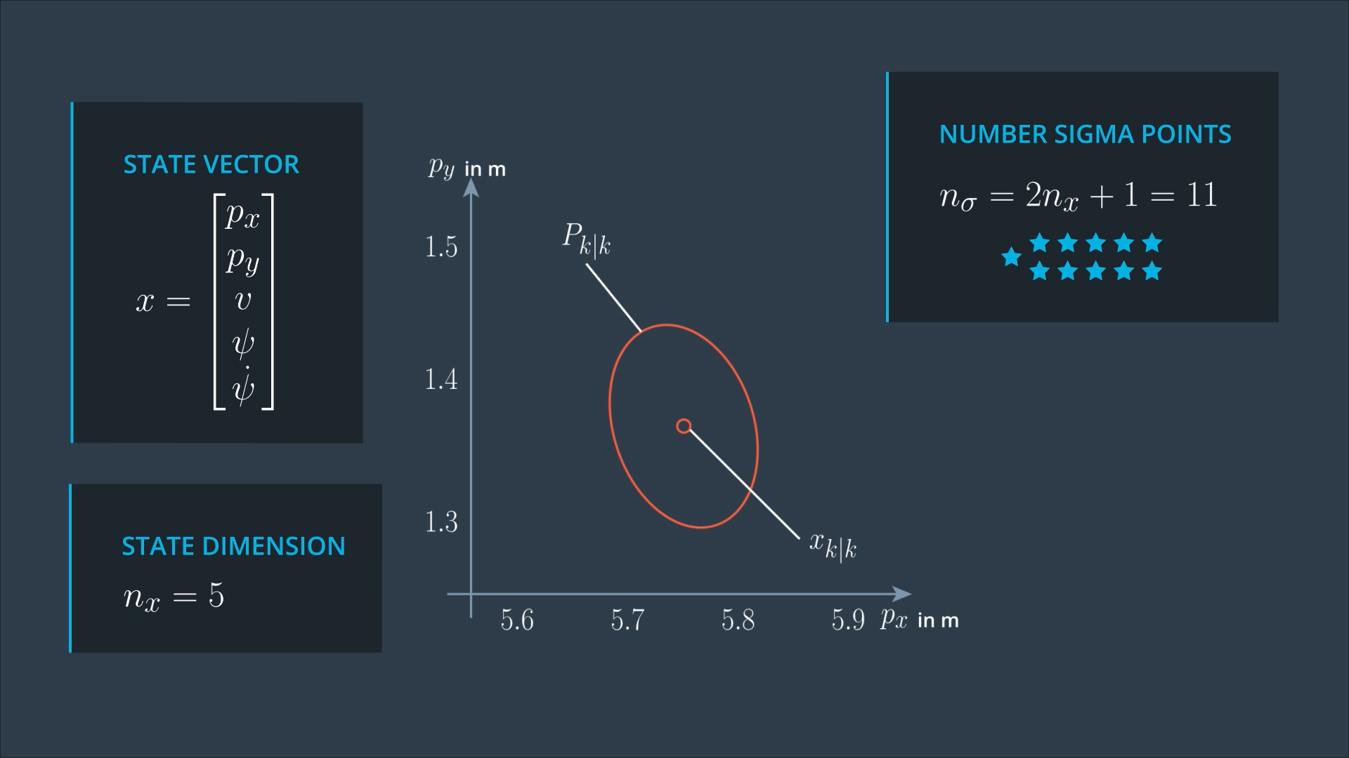
For simplicity, we will consider only 2 dimensions of our state vector px and py.

So, now we are looking for only 5 Sigma points.

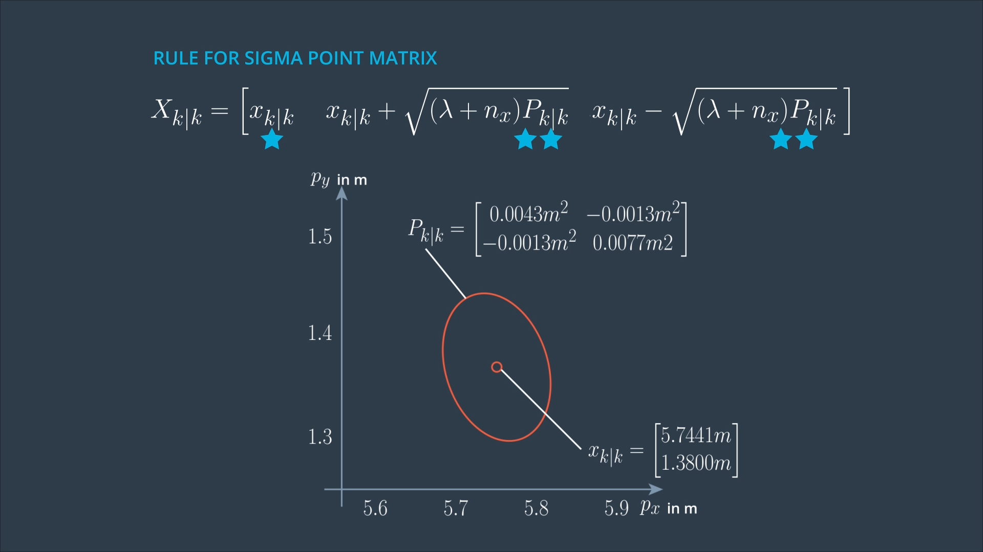
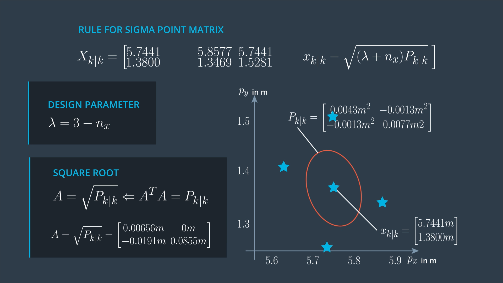
Lambda is a design parameter, which determines where in relation to the error ellipse you want to put your sigma points. Some people report good results with Lambda = 3 - nx.

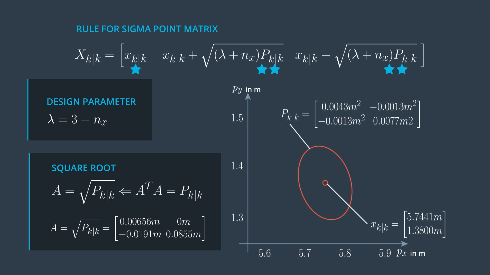
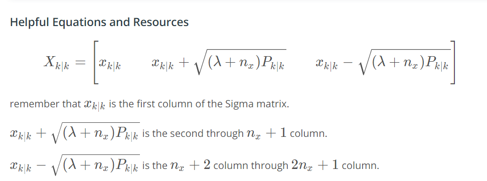
The first column of the matrix tells us what the first Sigma point is. This is always easy, because the first sigma point is the mean state estimate.

In the square root matrix, we have 2 vectors, and these two vectors are multiplied by a factor (Lambda + nx). If Lambda is larger, the sigma point moves further away from the mean state. If Lambda is smaller, the Sigma point moves closer to the mean state. This all happens in relation to this error ellipse.

Eigen: Quick reference guide

The Eigen library is divided in a Core module and several additional modules. Each module has a corresponding header file which has to be included in order to use the module. The Dense and header files are provided to conveniently gain access to several modules at once.

https://eigen.tuxfamily.org/dox/group__QuickRefPage.html

Eigen: Eigen::LLT Class Template Reference

Standard Cholesky decomposition (LL^T) of a matrix and associated features. Template Parameters _MatrixType the type of the matrix of which we are computing the LL^T Cholesky decomposition _UpLo the triangular part that will be used for the decompositon: Lower (default) or Upper. The other triangular part won't be read.

https://eigen.tuxfamily.org/dox/classEigen_1_1LLT.html

UKF Augmentation

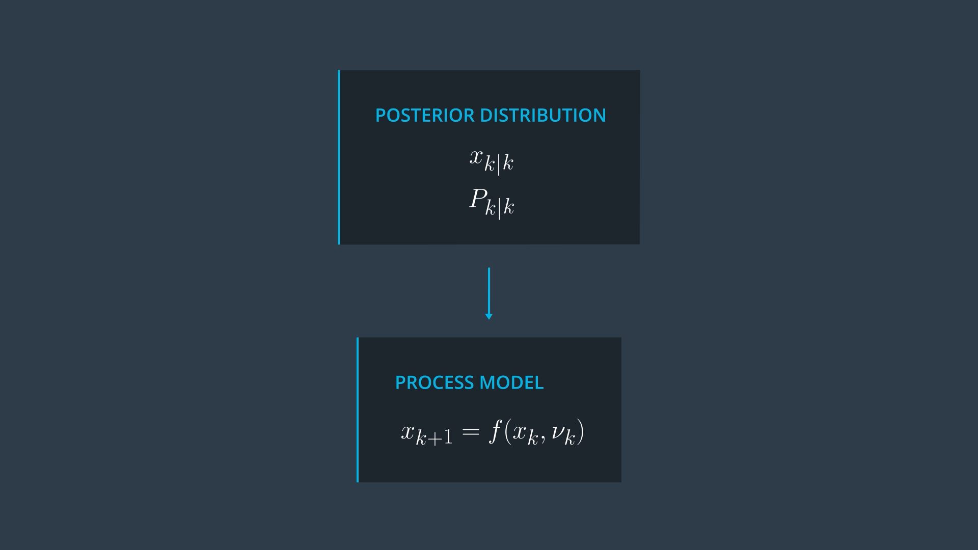
The process function also considers the process noise vector which also has a non linear effect.

UKF provides an easy way to handle non linear process noise effect.

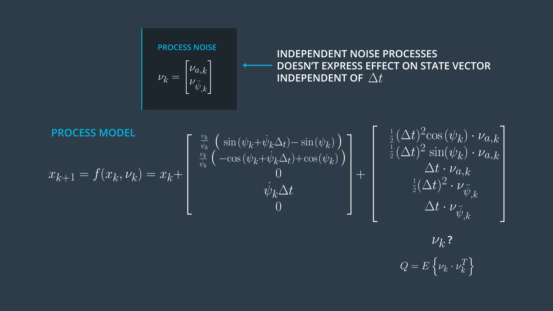
Each row of the last vector tells the influence of the process noise on a specific state between k and k+1, so it has the same dimension as the state vector and it depends on delta t.

In literature, authors may mention mu_k and mean the vector at the left (mostly this is the case when you read about standard linear kalman filter) or may mean the vector at the top. In the course we will stick with the last notation (which is much simpler, because this vector just lists the individual independent noise processes - This is mostly what authors mean when they write about unscented kalman filters).

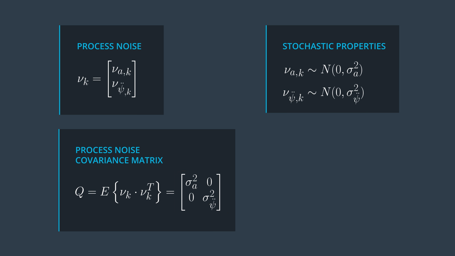
The covariances of the noise matrix Q are Zero, because the longitudinal acceleration noise and the yaw acceleration noise are considered independent.

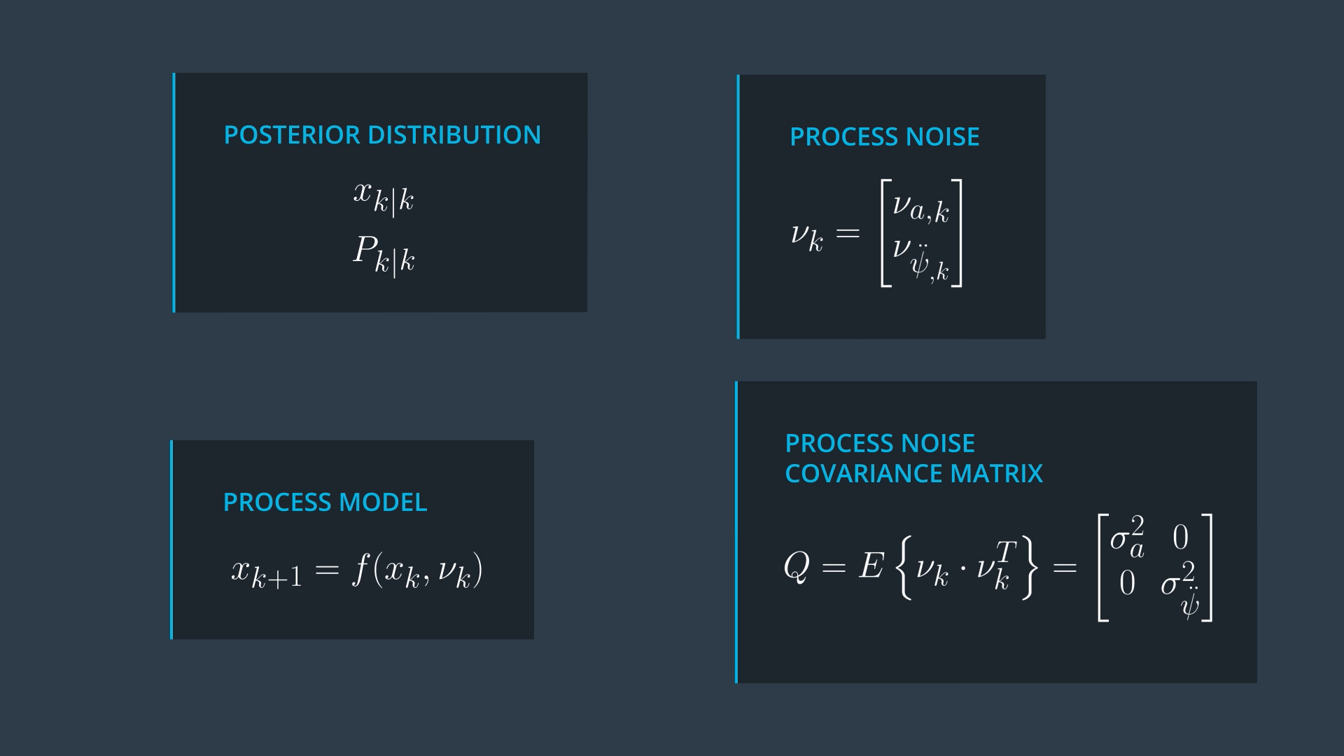
How to represent the uncertainty of the covariance matrix Q with sigma points?

→ The solution is called augmentation. We add the noise vector to the state vector. We need 15 sigma points now instead of 11.