Working with Real PCD

• Apply skills to actual point cloud data from a self-driving car.

• Do additional filtering techniques.

• Create a pipeline to perform obstacle detection across multiple streaming pcd files.

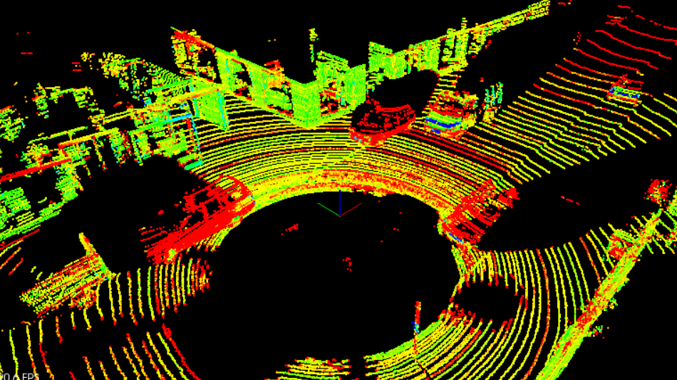
• Looking around the pcd, you can see several cars parked along the sides of the road and a truck approaching to pass the ego car on the left side. The goal will be to fit bounding boxes around these cars and the passing truck, so then your system could later use that information in its path planner, trying to avoid any collisions with those obstacles.

• Note: If the color is not specified in the renderPointCloud function argument, it will default to using the intensity color coding.

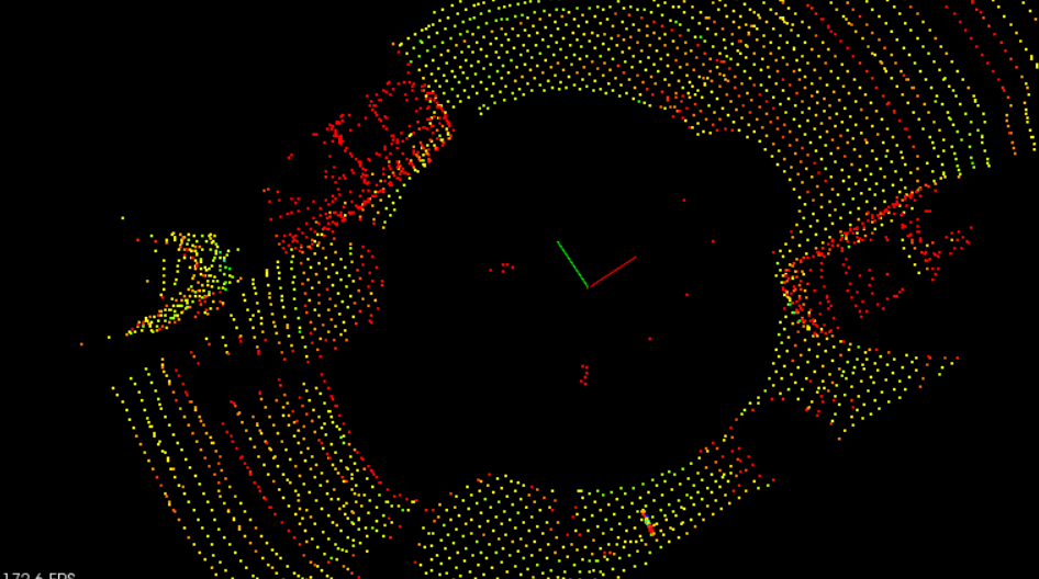
• The first thing you might notice when looking at the previous loaded point cloud is it’s quite high resolution and spans a pretty far distance. You want your processor pipeline to be able to digest point cloud as quickly as possible, so you will want to filter the cloud down.

Challenges with Real World Lidar

• Environmental Conditions: → Lidars do not do well in heavy rain, in whiteouts, brownouts (where there is a lot of dirt in the air, sand storms). Anything that reflects and scatters the laser beams of lidar in the air limits the its use. → Sometimes you create ghost objects (creating an object where there is no object) based on reflections (in case of highly reflecting surface). → You can also get lidar returns from spray. When it starts raining hard, you can have all kinds of weird objects as a result of the water that was spraying up from the tires from other cars.

Down-sampling Lidar Data

Sending out the entire point cloud over an internal vehicle network is a lot of data. As a result, we convert the point cloud into stixels (like what is done with stereo camera). Stixels are basically like a match. If you have the back of a vehicle, then stixels would be putting a bunch of match sticks to cover the vehicle. This gives you 2 things: 1- Number of match sticks (each one is lets say 4 inches wide) gives you the width of the vehicle. 2- The height of the match stick gives you the height of the vehicle. But you don't need anything in between, you just need the height and the width, and this reduces the data a lot and makes things easier to work with.

Filtering PCD

The fewer points we've, the faster processing. → We care about objects in our proximity Lidar can pick up things as far as 120 meters our from the very edge of our scene and not all of that is going to be completely relevant.

→ What is important? The width of the road (maybe 30 meters our from the front of the car and 10 meters from behind, since behind is not as important as the front).

→ Box region The box regions contain things that are in proximity and we want to label them as obstacles. We don't want to have any collisions with them.

Voxel Grid Filtering

A voxel is a 3D pixel (also called a volume pixel). It uses a lot less memory to describe it.

→ Voxel grid filtering will create a cubic grid and will filter the cloud by only leaving a single point per voxel cube, so the larger the cube length the lower the resolution of the point cloud.

→ The bigger our grid size (cell size), the fewer points we are going to end up with (every cell can only have one point).

Region of Interest

A boxed region is defined and any points outside that box are removed.

To apply these methods you will fill in the point process function FilterCloud. The arguments to this function will be your input cloud, voxel grid size, and min/max points representing your region of interest. The function will return the downsampled cloud with only points that were inside the region specified.

Steps For Obstacle Detection

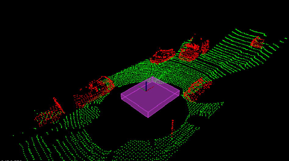
Step 1. Segment the filtered cloud into two parts, road and obstacles.

After you filter the point cloud the next step is to segment it. The image below shows the filtered point cloud segmented (road in green), (obstacles in red), with points only in the filtered region of interest. The image also displays a purple box showing the space where the car's roof points were contained, and removed.

Step 2. Cluster the obstacle cloud

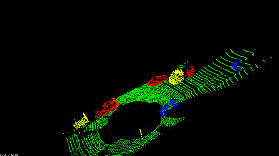
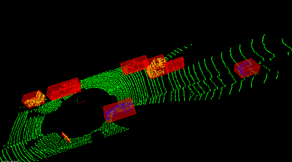
Next you cluster the obstacle cloud based on the proximity of neighboring points. The image below shows the clusters in cycled colors of red, yellow, and blue. In that image we see that the oncoming truck is actually broken up into two colors, front and back. This illustrates the challenges with clustering based on proximity, the gap between the front of the truck and the back of the truck is large enough so that they look separate. You might think to fix this by increasing the distance tolerance, but you can also see that the truck is getting really close to one of the side parked cars. Increasing the distance tolerance would run the risk of the truck and parked car being grouped together.

Step 3. Find bounding boxes for the clusters

Finally you place bounding boxes around the individual clusters. Since all the detectable vehicles in this scene are along the same axis as our car, the simple already set up bounding box function in point processor should yield good results.

Stream PCD

In the previous concept you were able to process obstacle detections on a single pcd file, now you are going to be using that same processing pipeline on multiple pcd files. To do this you can slightly modify the previous used cityBlock function from environment.cpp to support some additional arguments. Now, you will be passing in the point processor to the cityBlock function, this is because you don't want to have to recreate this object at every frame. Also the point cloud input will vary from frame to frame, so input point cloud will now become an input argument for cityBlock. The cityBlock function header should now look like this, and you no longer create the point processor or load a point cloud from inside the function.

void cityBlock(pcl::visualization::PCLVisualizer::Ptr& viewer, ProcessPointCloudspcl::PointXYZIpointProcessorI, const pcl::PointCloudpcl::PointXYZI::Ptr& inputCloud)

• Notice that in the function header you can optionally make inputCloud a constant reference by doing const and & at the end of the variable definition. You don't have to do this but you are not actually changing the inputCloud at all, just using it as an input for your point processor function. The benefit of using a constant reference is better memory efficiency, since you don't have to write to that variable's memory, just read from it, so it's a slight performance increase. If you do make this a const reference though, make sure not to modify it, or else you will get a compile error.

Code inside main

So now instead of creating your point processor, and loading pcl files from inside cityBlock you will do this inside the main function in environment.cpp right after where the pcl viewer camera position is set up.

ProcessPointClouds<pcl::PointXYZI>* pointProcessorI = new ProcessPointClouds<pcl::PointXYZI>();
std::vector<boost::filesystem::path> stream = pointProcessorI->streamPcd("../src/sensors/data/pcd/data_1");
auto streamIterator = stream.begin();
pcl::PointCloud<pcl::PointXYZI>::Ptr inputCloudI;

In the code above, you are making use of a new method from point processor called, streamPcd. You tell streamPcd a folder directory that contains all the sequentially ordered pcd files you want to process, and it returns a chronologically ordered vector of all those file names, called stream. You can then go through the stream vector in a couple of ways, one option is to use an iterator. At the end of the above code block, a variable for the input point cloud is also set up.

PCL Viewer Update Loop

The final thing to look at is the pcl viewer run cycle which is down at the bottom of envrionment.cpp. while the pcl viewer hasn't stopped, you want to process a new frame, do obstacle detection on it, and then view the results. Let's see how to set up this pcl viewer run cycle method below.

while (!viewer->wasStopped ())
{

  // Clear viewer
  viewer->removeAllPointClouds();
  viewer->removeAllShapes();

  // Load pcd and run obstacle detection process
  inputCloudI = pointProcessorI->loadPcd((*streamIterator).string());
  cityBlock(viewer, pointProcessorI, inputCloudI);

  streamIterator++;
  if(streamIterator == stream.end())
    streamIterator = stream.begin();

  viewer->spinOnce ();
}

The first thing the above method does is clear any previous rendered point clouds or shapes. Next it loads up your point cloud using your point processor and stream iterator. Then it calls your cityBlock function, and updates the iterator. If the iterator hits the end of the vector it simply sets it back to the beginning and that's it. The viewer->spinOnce() call controls the frame rate, by default it waits 1 time step, which would make it run as fast as possible. Depending on how timing efficient your obstacle detection functions were set up the faster the viewer's frame rate will be. If you want to check out the input pcd data at the fastest rate then run the code above and only run a single renderPointCloud on the input cloud inside cityBlock. Let's check out the results of the streaming pcd viewer below.